Voxel terrain: physics

In the last article we’ve discussed the particulars of voxel data definition and storage for voxel terrain we use at Roblox. From there on a lot of other systems read & write data from the storage and interpret it in different ways - the implementation for each system (rendering, networking, physics) is completely separate and not tied too much to decisions storage or other systems are making, so we can study them independently.

While logically speaking it would make sense to look at mesher next (which is how we call the component that is capable of taking a box of voxel data and producing triangle data representing the terrain surface with material attributes), since it is used by both physics and rendering systems, the algorithm is pretty involved and has quite a bit of “magic” so we will leave that for some other time and will instead look at physics today.

Initial prototype

Physics support is crucial for terrain since so much content we have relies on having robust physics behavior, both in-game and in-editor. For terrain in particular, having physics support meant implementing collision detection between terrain and all other shapes we use, as well as supporting raycasts efficiently. We care about performance and memory consumption, as the assumption is that some worlds will be heavily relying on terrain, including terrain physics.

While our physics engine is custom, we use some components of Bullet Physics for broadphase/narrowphase (specifically for complex convex objects and convex decomposition, relying on Bullet’s GJK implementation and some other algorithms), so it made sense to start by prototyping the solution that would heavily rely on Bullet.

Similarly to voxel storage, we divide the entire world into chunks and represent each chunk as a collision object; this division is crucial because each chunk becomes the unit of update of physics data - since terrain can be changed at any time, the chunk size is a balance between update cost (if a chunk is too big then every time we update a voxel in that chunk we’d have to pay a high cost of updating the entire chunk - we currently assume that incremental updates are too complex to implement as voxel changes can lead to changes in topology of the resulting mesh) and chunk overhead (if a chunk is 2^3 voxels, then we’d need to spend a lot of time/memory managing chunks). We settled on 8^3 chunks (as a reminder, a character is slightly taller than 1 voxel, which should give you a sense of scale) as a balance between these factors.

While we could try to do collision directly using the underlying voxel representation, the meshing algorithm we use is complex and makes it hard to accurately predict where the surface will be without running the algorithm; since our voxels are pretty big we wanted rendering and physics representation to match closely to eliminate visual artifacts so we decided to use the polygonal representation for collision.

Thus, the prototype took each chunk, ran mesher on the chunk to generate a triangle mesh from it, and then created a Bullet collision object using btBvhTriangleMeshShape. The resulting objects were inserted into the general broadphase structure along with other objects in the world; whenever an object, say, a ball, intersected one of the chunks, we would generate a contact object and then run Bullet’s algorithms to determine the contact points.

While this prototype got us going, it highlighted several key areas of improvement:

• Broadphase data is too imprecise - whenever any object intersects a 8^3 voxel chunk, we need to run narrowphase algorithm on the contact; this results in a lot of redundant contacts that don’t generate any contact points, especially in caves where an object hanging in mid-air can overlap with a relatively large chunk bounding box but never touch any geometry
• Narrowphase data is too large - for each chunk we end up storing the triangle mesh that is less compact than the voxel data (since we need to store vertex positions/indices) and Bullet’s BVH structure that is used to accelerate collision, which is also pretty large
• Narrowphase data is too slow to generate - while our meshing algorithm is heavily optimized, Bullet’s processing of the resulting mesh is relatively slow (up to 3x slower than generating the mesh)

This suggested that we need to change our approach for both broadphase and narrowphase. Let’s look at what we ended up doing there.

Bit broadphase: construction

Since the key issue with the broadphase was precision, we decided to teach broadphase about the structure of each object and do early rejects based on the actual voxel data - whenever an object moves, instead of creating a contact with each overlapping chunk, we would first look at the voxel data in the chunk to see if the object’s AABB intersects any voxel data.

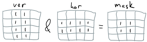
While our voxel data is pretty compact, we wanted to bring the memory impact of the broadphase data to the minimum. Additionally, the way our meshing algorithm works is that the geometry generated from a single voxel isn’t contained within that voxel and can spill into the neighboring voxels, so we actually need to check neighboring voxels as well. For all of this to work efficiently, we decided that for each chunk we would store a bitmask (where each voxel would correspond to one bit) that would tell us if each voxel has any geometry to collide with or not.

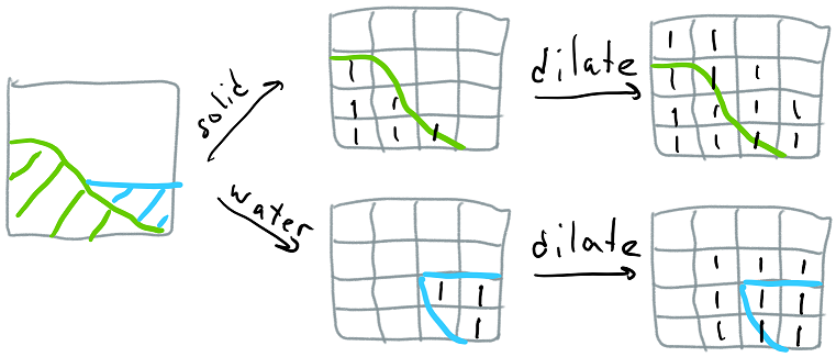
It’s vital to be able to generate this mask without relying on the meshing algorithm (since running the meshing algorithm on the entire terrain is too time consuming, and the way our code is structured broadphase data has to be available for the entire world), so we approximate this by saying that if a voxel is solid, it can in theory generate geometry inside any of its neighboring voxels (including diagonal neighbors, for a total of 3^3=27 voxels), and fill all of these voxels with 1s in the mask - this process is called dilation. This also requires that we look at the neighboring voxels of the chunk, so our input is a 10^3 voxel box and our output is a 8^3 bitmask.

Finally, we have two types of contacts - solid and water (we use contacts between primitives and water to compute buoyancy), so we generate two bitmasks. The process works roughly as follows (note that for exposition the images in this article are assuming 4^3 chunks instead of 8^3):

To make this process fast, we dilate using bit operations - we first generate the 10^3 bitmask and store it in an array of 10^2 16-bit integers, then we dilate each integer horizontally like this:

data[y][z] = (data[y][z] << 1) | data[y][z] | (data[y][z] >> 1);

Then we dilate along other two axes in two passes like this:

temp[y][z] = data[y][z - 1] | data[y][z] | data[y][z + 1];

As a result, we get 10^2 10-bit dilated bitmasks; we then extract 8^2 8-bit bitmasks that correspond to chunk’s voxels (discarding the redundant boundary voxels) and store them as the broadphase data. During this process we also filter out redundant chunks - if all voxels in the 10^3 volume are filled with air then there’s no geometry there; also, if all voxels in the 10^3 volume are filled with either a solid material or water, then our meshing algorithm will never generate any polygons but we still need to keep this chunk in the broadphase (for example, to be able to tell if an object is fully submerged in water) so we tag it in a special way.

Overall, this results in extremely low storage costs - the worst case is 2 bit/voxel (1 bit for solid mask and 1 bit for water mask), but many chunks are discarded since they are either empty or full and in this case we just need to store the chunk structure but not the mask.

Bit broadphase: overlap test

Now that we’ve generated the broadphase data (this is done when the level loads and each chunk’s broadphase data is regenerated whenever any voxel in a chunk changes), we can look at how we use it.

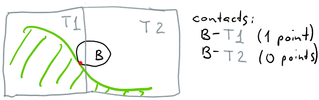
Whenever the object moves, we take the AABB of the object with the old and new transforms, query the broadphase for overlaps and perform contact management - if the object had a solid contact with a chunk in the old position but no solid contact with that chunk in the new position, we can remove that contact. We track up to 1 solid and 1 water contact per object-chunk pair, so a very large object can end up having multiple contacts with terrain (and each contact can generate multiple contact points as a result of the narrowphase work that we’ll discuss later).

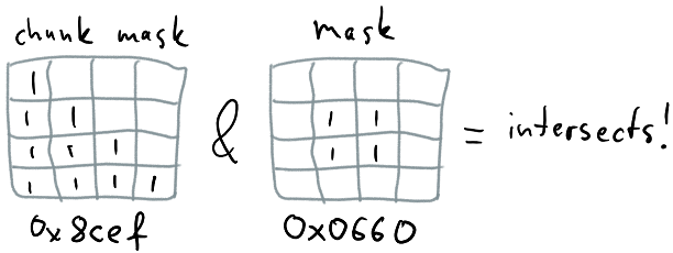
The query is two-step - first, we take the object’s AABB, expand it by 1 voxel to cover for objects touching geometry generated by overflowing into the neighboring voxel, project it to chunk space (by dividing the coordinates by 8 voxels), and convert the min/max to integer (using floor/ceil), which gives us the range of chunks. Then we take each chunk and inspect the bit data to see if the object’s AABB touches any bits marked as solid/water. While the latter could be implemented in a naïve way by querying each voxel in the object’s AABB, we take advantage of the bit data as follows.

Remember that we have 8^3 bits in a chunk; we store each Y-slice (Y points up) of this chunk in a 64-bit integer, with each successive group of 8 bits determining the data for a X-row. Each mask is thus a simple array, and we store one mask for solid and one mask for water:

uint64_t solid[8];
uint64_t water[8];

Now, we take the object’s AABB, we project it to the chunk space and determine the bounds in voxel space. Then, we look at object’s XZ extents as it intersects the chunk and generate a 64-bit mask that has 1s set where the object intersects voxels along XZ plane:

Then we iterate through all Y-slices that the object covers, and do a simple bit test for each slice:

if (chunk.solid[y] & mask)
    touchesSolid = true;

This lets us check the entire XZ slice of a chunk - up to 64 voxels! - for overlap with a simple instruction (on 32-bit architectures this test takes ~3 instructions), which makes it very efficient to do precise queries on reasonably large objects. To optimize the overhead for small objects, we make sure to create the mask for the XZ extents as fast as possible - while we could do it by iterating through XZ extents and setting bits, we note that the mask we have is really an intersection of two masks representing one vertical strip and one horizontal strip; for each direction we keep a lookup table and combine the lookup results to get the resulting mask:

uint64_t mask = masksVer[cmin.x][cmax.x] & masksHor[cmin.z][cmax.z];

Narrowphase: analysis & plan

Now that we have our broadphase data in good shape, let’s look at narrowphase. On a high level the way Bullet-based narrowphase worked was as follows:

• Each chunk stores an array of vertices (each vertex has 3 floats for position and 1 byte for material), an array of indices (each triangle has 3 16-bit indices) and a BVH (which is an AABB tree)
• When creating the tree, the list of triangles would get repeatedly subdivided into nodes up until the leaf nodes have just one triangle
• When performing collision detection, a set of triangles is extracted from the tree using a simple AABB query; each triangle gets collided with the target primitive using either a specialized algorithm for this pair (like triangle-sphere) or a generic GJK/EPA algorithm. The points resulting from these collisions are fed into a simplex structure that keeps up to 4 contact points and tries to maximize contact area
• When performing raycasts, a simple ray-AABB tree query is ran; each matching leaf node is intersected with the ray. The closest point is kept and returned as the result.

We decided to keep the collision detection algorithms and the overall structure, but replace all other components with versions that worked better for our use case. To keep the memory cost low, we started doing lazy generation of collision objects - we would only generate triangle/tree data when a contact was created or a raycast against the chunk was performed, and would keep a cache of the resulting objects so that the memory overhead remained manageable.

This significantly improved narrowphase memory consumption, but the generation cost remained prohibitively expensive. Bullet has two versions of their BVH triangle mesh tree: a non-quantized one and a quantized one. Each keeps an AABB tree but stores them differently (with 32-bit floating point in one case, and 16-bit integer in another). Since each triangle has a leaf node and the tree is binary, you need about twice as many nodes as you have triangles.

The base memory cost for a raw mesh is ~13b per vertex (3 floating point coordinates and 1 byte material) and ~6b per triangle (for 3 16-bit indices), which adds up to ~12.5b/triangle since on average there are twice as many triangles as vertices.

The non-quantized Bullet BVH takes 64 bytes per node which adds up to ~128b/triangle (the node structure only needs 44 bytes but it’s padded to 64 bytes), which is ~10x the memory cost of triangle data. The tree also takes ~3x longer to generate compared to generating the mesh (using our implementation that converts voxel data to triangle data).

The quantized Bullet BVH takes 16 bytes per node which adds up to ~32b/triangle, which is ~2.5x the memory cost of triangle data. It is slower to generate compared to non-quantized version, around ~5x longer compared to generating the mesh.

Both of these options were very unsatisfactory in terms of both memory and time to generate the data (due to lazy generation the construction time is important), so we decided to replace the tree structure with a custom kD tree with two planes per node.

Loose kD tree: construction

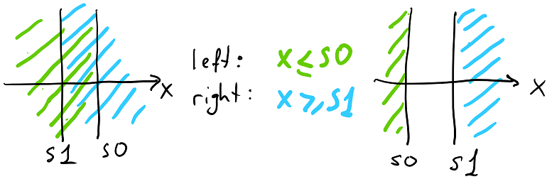
The kD tree is a binary tree with each node splitting the space along one axis in two parts. Usually kD tree only has one splitting plane per node, but this makes dealing with triangles that aren’t contained completely within one of the children complicated (you have to cut them with the splitting plane), so we settled on a loose kD tree - each node has two splitting planes along the same axis, where all left children are contained within a subspace defined by one of them, and all right children are contained within a subspace defined by the other one. The planes tightly fit the content of child nodes, resulting in two possible plane configurations:

While an AABB tree can localize the space a bit better than kD tree in general, kD tree can be faster to construct and you can recover most of the information during the recursive traversal as we’ll discuss later. The big benefit is that you only need to store 2 values per node instead of a full AABB. We also decided to store more than one triangle per leaf node - in general storing 2 triangles instead of 1 does not significantly affect the query quality - and ended up with this structure:

union KDNode {
    struct {
        float splits[2];
        unsigned int axis: 2; // 0=X, 1=Y, 2=Z
        unsigned int childIndex: 30; // children are at childIndex+0,1
    } branch;

    struct {
        unsigned int triangles[2]; // up to two triangles per leaf
        unsigned int axis: 2; // must be 3; same offset as branch.axis
        unsigned int triangleCount: 30;
    } leaf;
};

The tree structure is relatively straightforward; all nodes are stored in one large array so that we can refer to nodes using an index. The 4-th value of axis index is used as a tag to distinguish leaves, and just one child index is stored since each branch node always has both children. We store up to 2 triangles in each leaf node; we easily have space for 4 but storing 4 triangles instead of 2 was slightly slower to process collisions for so we went with 2.

Note that the node is 12 bytes and since we store 2 triangles in each leaf node, we need around as many total nodes as we have triangles, so the memory cost ends up being 12b/triangle. There is absolutely more room for optimization here as well - we could reduce the memory cost for vertex data by packing positions using 16-bit integers and optimize the kD tree node in a similar fashion, getting to ~6b per kD node and resulting in total triangle impact of 3.5b vertex + 6b index + 6b tree = 15.5b, but the current result of ~24.5b/triangle was good enough to ship.

The process of tree construction is relatively standard - we start with an array of triangles, and recursively subdivide it, generating branch nodes in the process (and stopping the recursion once we reach 2 triangles per node or less). For each division we pick the axis by taking the longest axis of the current AABB, place the split point at the average of triangle midpoints along this axis, filter triangles to the left/right of that plane using their midpoints as the decision factor and then recompute the left and right split planes using all 3 triangle vertices. If the resulting distribution ends up too skewed in terms of triangle counts (this is currently defined as <25% of triangles ending up in one of the two nodes), we repartition and put half of the triangles in one subtree and half in another subtree (out of the list sorted by midpoints) - this maintains a balance between spatial coherency and tree depth, limits the tree depth and makes sure the process terminates.

The construction process ends up being a bit simpler and is coded more efficiently than Bullet’s, and thus is ~3-4x faster than the Bullet’s fastest tree construction algorithm. This results in mesh & tree data being roughly equivalent in size and roughly equivalent in generation time, which is a good balance (or rather this means that to make significant improvements in the overall process you need to significantly optimize both :D).

Loose kD tree: queries

As mentioned before, we only need two types of queries - AABB query (where we need to gather all triangles contained within a given AABB, which is used for narrowphase) and raycast query (where we need to gather all triangles intersecting a ray, or just the one with the closest intersection point). Both of these are implemented using stackless traversal - since the tree depth is bounded, it’s easy to precompute the tree depth and preallocate scratch space for the given traversal. Stackless traversal doesn’t necessarily save us much space or time, but it helps understand the profiling results since all overhead from the traversal in both branches and leaves is centralized in one function, making it somewhat easier to work with.

kD tree doesn’t have the full knowledge about the node extents in each node, like AABB tree, but we can recover it during the traversal. For AABB query when we encounter a branch node, we only descend down the branches that have the AABB in the right half-space; due to the hierarchical traversal this ends up only traversing the nodes with volume overlapping the AABB:

if (node.branch.splits[1] <= aabbMax[axis])
    buffer[offset++] = childIndex + 1; // push right child

if (node.branch.splits[0] >= aabbMin[axis])
    buffer[offset++] = childIndex + 0; // push left child

This can be inefficient if the queried AABB is outside of the full kD tree bounds so we store an AABB for each kD tree for early rejection.

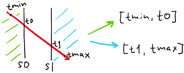
For ray queries, we choose to instead do a segment-tree traversal, where the segment is defined by the ray origin/direction and two limits for the parameter t, tmin and tmax, that contain all points within the subspace defined by each node. When we encounter a branch, we need to intersect the split planes with the ray (which is simple & fast since planes are axis-aligned), and adjust the t limits for subsequent traversal:

float sa = raySource[axis];
float da = rayDir[axis];

float t0 = (node.branch.splits[i0] - sa) / da;
float t1 = (node.branch.splits[i1] - sa) / da;

if (t1 <= rn.tmax)
    buffer[offset++] = { childIndex + i1, max(t1, rn.tmin), rn.tmax };

if (t0 >= rn.tmin)
    buffer[offset++] = { childIndex + i0, rn.tmin, min(t0, rn.tmax) };

Similarly to AABB queries, if the ray doesn’t intersect the full kD tree bounds the traversal can be inefficient, so we compute the initial segment limits by intersecting the ray against the stored AABB.

Additionally, to accelerate ray queries that just need the first point, we arrange the traversal to first visit the branch that defines a subspace that occurs earlier along the ray’s direction (this affects i0/i1 indices in the snippet above); if we find an intersection point that is earlier along the ray than the minimum t of a given segment then we can terminate the traversal. Unfortunately, due to floating point precision issues we need to slightly expand the segment on each branch.

With this we get efficient tree queries for both AABB and raycasts; the AABB query performance is on par with Bullet implementation, but the raycast query is faster, both because we do less work for each branch (only intersecting two planes with a ray), and because we can terminate the traversal early if we found a suitable intersection point.

Future work

While the resulting algorithms we’ve built work pretty well, they can undoubtedly be improved even further. Memory consumption of narrowphase could be improved; additionally we currently store triangles in the kD tree - Christer Ericson suggested that if you store quads as a first class primitive, the raycasts can be up to 2x more efficient since Möller-Trumbore algorithm can handle quads with minimal additional computation (our terrain is built using quads, and some of them are planar, so this could be viable).

One area that we have yet to explore is the parts of narrowphase that we still use from Bullet. It’s possible that one can utilize better algorithms for doing triangle-convex collisions or for reducing the contact point manifold, and additionally we currently use a few hacks to deal with interior edge collisions whereas we could generate the data about whether each edge is exterior or interior and use this when generating collision points/normals.

Finally, something that we have explored during the prototyping phase but didn’t get into production is disjoint terrain regions - whenever you modified voxel data our prototype performed a basic connectivity analysis and converted all disjoint connected voxel regions into a freely moving object. Computing collisions for this in real-time most likely involves approximating the shape with a convex hull, although other options might be possible and we will probably explore this one day.