Learning from data

Machine learning is taking the world by storm. There’s amazing progress in many areas that were either considered intractable or had not reached a satisfying solution despite decades of research. A lot of results in machine learning are obtained using neural networks, but that’s just one class of algorithms. Today we’ll look at one key algorithm from meshoptimizer that was improved by getting the machine to find the best answer instead of me, the human¹.

Problem

One little known fact is that the performance of rendering a mesh depends significantly on the order of triangles in that mesh. Most GPUs use a structure that we will call “vertex cache” (also known as “post T&L cache”, “post transform cache” and “parameter cache”) which can cache the results of the vertex shader invocation. The cache is indexed by the vertex index, and the details of the cache replacement are not documented and vary between GPU vendors and models.

For example, if the triangle [2 1 3] immediately follows a triangle [0 1 2] in the index buffer, it’s very likely that the vertices 1 and 2 will not be transformed redundantly. However, if there are a lot of other triangles between these two in the index buffer, the GPU might need to transform these vertices again. Minimizing these redundant vertex shader invocations (cache misses) is beneficial for performance.

There are many ways such a cache could function; a few obvious models are a fixed-size FIFO cache and a fixed-size LRU cache. Existing hardware mostly doesn’t follow any of these; specifically for fixed-size FIFO, relying on the replacement policy can be dangerous as illustrated by Optimal grid rendering isn’t optimal.

However, even if we knew the replacement policy for our target hardware, what would we do with this information? Problems of this nature tend to be NP-complete and require some sort of heuristics to get a reasonable result in finite amount of time.

Algorithms

There are a few well known algorithms for optimizing meshes for vertex reuse. Two algorithms that I’ve implemented for meshoptimizer are Tipsy, which models a fixed-size FIFO cache, and Tom Forsyth’s Linear-Speed Vertex Cache Optimisation , which models a fixed-size LRU cache.

Both algorithms are greedy and work a bit similarly - given a set of recently seen vertices, they look at the adjacent triangles (TomF) or vertices (Tipsy), pick the next one, and emit the triangle or adjacent triangles. The selection of the next triangle is optimized to try to improve the overall cache efficiency.

Coming up with a heuristic that doesn’t compromise the global order in favor of the local order is challenging, since the heuristic only looks at the next possible choice². This is especially hard since the details of the cache behavior aren’t known.

Initially after implementing both algorithms, I was tempted to abandon TomF’s algorithm. Using a fixed-size FIFO cache, Tipsy was generally producing slightly more efficient results on most meshes, substantially more efficient results on some meshes, notably large uniform grids, and was several times faster to boot - which isn’t that big of a deal until you are dealing with meshes that have millions of triangles. However, what if the hardware isn’t using a fixed-size FIFO³?

Evaluation

Instead of using a simple FIFO model when evaluating the algorithms, I decided to compare the behavior on the actual hardware.

There are a couple of ways to do this - notably, you can use unordered access from vertex shaders to try to measure the number of times each vertex gets transformed, or use performance counters provided by the hardware to measure the vertex shader invocation count. I implemented a simple program that used the performance counters and ran it on a few test meshes.

The results were surprising. On both NVidia and AMD hardware, on the meshes where Tipsy was doing comparably or slightly better on the FIFO cache misses, the hardware counters consistently showed that TomF⁴ was generating a noticeably more efficient order - with the exception of uniform grids.

First I wanted to understand the hardware behavior better. While it’s straightforward to compute the total number of vertex shader invocations from an index sequence, it makes analysis cumbersome - this would tell us “this index sequence results in 19 invocations”, but won’t tell us why. To help with this a special analysis tool was written to measure invocation count on variants of the input sequence:

• For a given index sequence, we will compute the number of invocations for each prefix of the sequence that forms a triangle list; this means that for each triangle in the sequence, we can look at the sequence up until the previous triangle and determine the increase in the number of invocations from adding this triangle.
• In addition to that, to try to analyze the indices within the triangle better, we will look at variants of the sequence where we replace triangle a b c with a a a and a b b.
• Finally, to understand the state of the cache after processing the sequence, for each index i we will append the triangle i i i to the sequence and measure the resulting invocations⁵.

The reason why we need to perform the modifications of the sequence is so that we can try to understand which specific indices in the sequence are causing a cache hit or miss. For example, if we know that adding the triangle a b c increases the invocation count by 1, we can guess that only one of the indices results in an additional invocation; if replacing this triangle with a a a leaves the invocation count as is, but replacing it with a b b increases it by 1 as well, then it’s likely that we had to transform b and not a or c.

As a result, for a given index sequence we can produce the result that looks like this:

// GPU 1: NVIDIA GeForce GTX 965M (Vendor 10de Device 1427)
// Sequence: 120 indices
//   0*3:   1*   2*   3*   4*   5*   6*   7*   8*   9*  10*   1    2
//   4*3:   3    4    5    6    7    8    9   10    1    2    3    4
//   8*3:   5    6    7    8    9   10    1    2    3    4    5    6
//  12*3:   7    8    9   10    1    2    3    4    5    6    7    8
//  16*3:   9   10    1    2    3    4    5    6    7    8    9   10
//  20*3:   1    2    3    4    5    6    7    8    9   10    1    2
//  24*3:   3    4    5    6    7    8    9   10    1    2    3    4
//  28*3:   5    6    7    8    9   10    1    2    3    4    5    6
//  32*3:   7*   8*   9*  10*   1*   2*   3*   4*   5*   6*   7    8
//  36*3:   9   10    1    2    3    4    5    6    7    8    9   10
// Cached  : 1 2 3 4 5 6 7 8 9 10 (10)
// Invocations: 20

In this case, given a degenerate sequence of 12 1-10 index groups, we get 20 invocations - each vertex was processed twice - and we know which specific indices were processed (marked with *) and which weren’t. Now what we need to do is to analyze a number of index sequences to study the patterns and come up with a theory that explains them best.

I won’t go too much into the results of the analysis - while it’s an interesting topic on its own, I’m not sure what hardware vendors would think of this, and I later learned of a fantastic paper that did this analysis using similar methods, Revisiting The Vertex Cache: Understanding and Optimizing Vertex Processing on the modern GPU.

As a result, I had to enhance the simulation algorithms used in meshoptimizer to measure the efficiency of the resulting index sequences to support more configurable parameters so that I could quickly measure the efficiency of the resulting sequence on models that resemble NVidia, AMD and Intel. All three vendors use different parameters and replacement policies for their caches - if any of them are reading this, it would be nice if these details were publicly documented.

With that out of the way… how do we actually improve the results?

Scoring

The way TomF algorithm works is that every time it emits a triangle, it picks the triangle with the highest score from the set of candidates (that are adjacent to a few most recently seen vertices). The score of the triangle is the sum of the scores of the vertices, and the score of the vertex is determined from two numbers, cache (position of the vertex in LRU cache, 0 = most recent) and valence (the number of triangles that this vertex belongs to that haven’t been emitted yet) as follows:

• the score is the sum of cache score and valence score
• cache score is last_triangle_score if cache < 3 and ((cache - 3) / (cache_size - 3)) ^ cache_decay_power otherwise
• valence score is valence_boost_scale / (valence ^ valence_boost_power)
• last_triangle_score = 0.75, cache_decay_power = 1.5, valence_boost_scale = 2.0, valence_boost_power = 0.5

So generally speaking, the score decreases non-linearly as the cache position increases (the score is higher for recently seen vertices) and decreases non-linearly as the valence increases (the score is higher for vertices with fewer remaining triangles). Additionally, the score for three most recently seen vertices is artificially lowered to avoid the strip-like runs that penalize long-term efficiency.

The heuristic intuitively makes sense. However, is it the best heuristic possible? One of the known problems with it was the suboptimal performance on uniform grids. I wanted to solve this, but wasn’t sure how to do so - it’s hard to find local tweaks of this heuristic that result in more optimal behavior globally.

One obvious thought is that while the shape of the heuristic makes sense, it’s unclear that the parameters are chosen optimally. Why is the last triangle score 0.75 instead of, say, 0.8?

To try to explore this further I implemented a simple brute-force optimization algorithm: there are only 4 values, so we can reasonably explore many different combinations of the values, adjusting each parameter by a small increment, such as 0.05, and rerunning the algorithm on a test data set. If the resulting efficiency improves, we found constants that are slightly better.

After rerunning the tuning, I found slightly better values for the formula - last_triangle_score = 0.8, valence_boost_scale = 3.2, valence_boost_power = 0.9 - but the gains were marginal, ~1% relative improvement on simulated NVidia-like model.

Tables

One other problem of the original algorithm was performance. In order to make it as fast as I could without sacrificing the quality, I replaced the expensive power functions in the original formula with cheaper table lookups, resulting in tables like this:

// last_triangle_score = 0.8, cache_decay_power = 1.5
static const float vertex_score_table_cache[1 + max_cache_size] =
{
    0.000000f,
    0.800000f, 0.800000f, 0.800000f, 1.000000f, 0.948724f, 0.898356f, 0.848913f, 0.800411f,
    0.752870f, 0.706309f, 0.660750f, 0.616215f, 0.572727f, 0.530314f, 0.489003f, 0.448824f,
    0.409810f, 0.371997f, 0.335425f, 0.300136f, 0.266180f, 0.233610f, 0.202490f, 0.172889f,
    0.144890f, 0.118591f, 0.094109f, 0.071591f, 0.051226f, 0.033272f, 0.018111f, 0.006403f,
};

// valence_boost_scale = 3.2, valence_boost_power = 0.9
static const float vertex_score_table_live[1 + max_valence] =
{
    0.000000f, 3.200000f, 1.714838f, 1.190531f, 0.918959f, 0.751756f, 0.637990f, 0.555344f,
    0.492458f, 0.442927f, 0.402856f, 0.369740f, 0.341890f, 0.318127f, 0.297601f, 0.279684f,
    0.263902f, 0.249888f, 0.237358f, 0.226085f, 0.215885f, 0.206611f, 0.198139f, 0.190368f,
    0.183215f, 0.176605f, 0.170480f, 0.164787f, 0.159481f, 0.154523f, 0.149879f, 0.145521f,
};

After this I reduced the table sizes to 16 for cache and 8 for valence, since this didn’t seem to matter for the quality of the results, but reducing the simulated cache size substantially improved the performance of the algorithm.

One day I was staring at the tables and it suddenly hit me: if I am already evaluating the score as f(cache) + g(valence) and if f and g are already table-driven, why do I need to generate the tables from some preconceived formula with bruteforced parameters if I can just find the optimal tables?

Tuning

After the tables became smaller, the cache table had 16 floats between 0 and 1, and the valence table had 8 floats - they were originally outside of the [0..1] range but since the entire formula is scale-independent, we can normalize everything to [0..1]. This gives us 24 floats that we need to find.

For each set of 24 values we can take a data set with many representative meshes (the test sets I use vary a bit, my most recent set contains a uniform grid - this was important to improve! - and a collection of various meshes including scans, sculpts, high poly and low poly game-ready models, for a total of ~1M triangles), optimize them using the table-driven algorithm and then measure the results. The same process can then be applied to a larger control set to make sure we aren’t overfitting the parameters to the test data set.

To compare the results, I measured the data using models for multiple vendors (initially using Intel, NVidia and AMD) and computing the fitness function as a sum of relative improvements between the baseline and the optimized result for all meshes. This metric is independent of the triangle count in each mesh, which is good because it means that one high-poly mesh doesn’t get weighted more than meshes with fewer triangles.

Now that we can evaluate a given table… how do you bruteforce a 24-dimensional space?

I have repeated the optimization process several times in the last few years, experimenting with different algorithms. In each case I took a specific optimization algorithm and ran it using a many-core machine using OpenMP for parallelization⁶ (typically 64-core or 96-core cloud instance, ultimately paying hundreds of dollars to cloud providers) over a course of several days. To save costs when running on cloud, I ended up using Google Cloud instead of AWS EC2 because the compute prices were cheaper, and using preemptible instances to get 2-3x cheaper execution. Because the optimization has to run for multiple days, I implemented support for persisting state so that when the cloud VM gets shut down due to preemption the state isn’t lost; additionally a non-preemptible watchdog VM was running and constantly waking up the many-core VM every 5 minutes⁷.

96 threads sound like a lot, but 24 dimensions is just way too much. For each combination of 24 numbers we need to run a million triangles through the optimization algorithm and then compute the fitness function. This process isn’t very fast.

Optimization

To make the problem tractable, we need to use an optimization algorithm. I tried to use three different ones over the years.

First I implemented a genetic algorithm. Since our table is just a short vector of 24 floats, it’s trivial to implement mutation and crossover. Then you seed the population with many random vectors, and wait. And wait. And wait.

I don’t know if this was a good idea, but I was upset when after a round of evolution the next population wasn’t always better than the old one - that is, the best individual from one population could be replaced by a slightly worse one from the next population, and it wasn’t clear that the process should converge. To fix that the generic evolution cheated and picked the best few specimens out of the population and copied them to the new population verbatim; the rest were generated using mutation/crossover.

The results of the tuning process were extremely promising. Although it took many CPU hours to get there, the resulting table was better than the table I started with - in many cases the delta was noticeable but not very significant, except for uniform grids where the results were ~10% better than the previous table.

Additionally, this served as a validation for some of the intuition behind the heuristic used previously. The training was done tabula rasa - with no a-priori knowledge about the problem, and only given the framework for the solution (the separable vertex scoring function), the machine has decided that indeed, the three most recently seen vertices should have a lower score than others (even though it didn’t assign equal weights to all three, using 0.792f, 0.767f, 0.764f - of course there’s a fair bit of noise in the resulting values).

The optimization process seemed to get stuck after 3 days, and since I was paying real money for the experiments, I decided to try to alter the training algorithm in hopes that a different algorithm can produce better results.

The next algorithm I implemented was a variant of simulated annealing. Instead of performing mutation/cross-over, and arbitrarily picking some fraction of the last population as survivors, there’s a set of “temperature bands” and within each we can find a new state by mutating the old state, and probabilistically decide whether to replace the old state with the new one based on the difference in fitness.

The classical description of the algorithm suggests starting with a high temperature value and gradually “cooling” it off - when temperature reaches 0, the result stabilizes. This didn’t fit the desired behavior since I didn’t know how to tune the starting temperature and wanted the algorithm to run indefinitely, so instead the annealing is performed simultaneously for multiple temperature values, and at the end of the run the best state propagates from higher temperatures to lower temperatures. This gives similar continuity to the solution - the best result (the state of the temperature band 0) continuously gets better.

Of course, the algorithm eventually gets stuck as well. It is probably the case that it’s possible to get better results with annealing but the results of the genetic optimizer were superior.

At some point last year I was talking to Angelo and the subject of numeric optimization came up. He introduced me to differential evolution which, contrary to what you might expect from the name, doesn’t require the function to be differentiable. Using the basic formulation from Wikipedia and the set of parameters suggested in Good Parameters for Differential Evolution, I was able to improve on the results a little bit further - differential evolution running for a day on a 96-core GCP instance resulted in the final tables that are still used right now.

The beauty of the approach is that it just takes a little bit of machine time now to generate the functions for the target profile. For example, if somebody from AMD reached out to me tomorrow and told me exactly how the vertex reuse policy works (hint hint), I could generate a special table for AMD hardware that would probably be a few percent more efficient than the existing one - which might be reasonable to use when shipping a console title. Additionally, it’s much easier to explore a wider set of shapes of the heuristic function - maybe instead of adding the vertex scores we should multiply them? (nope) maybe we should generate a 16x8 non-separable table instead of 16+8 separable one? (haven’t tried this yet because of concerns about insufficient size of the data set) etc.

Compression

A lot of work I am doing lately involves finding ways to efficiently compress the vertex and index data - instead of implementing complex mesh traversal algorithms that take a while to run during decompression and penalize rendering efficiency, the algorithms start from a triangle order optimized for vertex reuse and try to compress that.

Specifically, meshoptimizer now ships with a index encoder (that assumes the index buffer has been optimized for vertex reuse, preserves the order, and outputs a much smaller byte sequence that can be decoded back into the index buffer at 1-2 GB/sec) and a stripifier (that starts with an optimized index buffer, and generates a sequence of triangle strips that tries to maintain reasonable reuse efficiency by slightly changing the triangle order but not too much in order to find a balance between vertex reuse and triangle strip length).

When rendering performance is crucial, the index buffer should be optimized for vertex reuse and then compressed; when VRAM size is crucial it may be worth optimizing the index buffer and then converting it to triangle strips.

What if it’s really important to optimize for compressed mesh size instead? Can we keep the overall algorithms and encoding structure, and produce a smaller compressed mesh? After exploring a few different ways to encode the index buffer differently while still maintaining the order perfectly, I kept running into the order restriction and it became obvious that to generate smaller meshes with this approach, it was critical to reorder triangles a bit differently.

If only there was a way to find a triangle order for a mesh that, instead of just optimizing for rendering efficiency, tried to make the index buffer - after using the specialized index compression - smaller.

Wait. Right. That’s what we just did.

Eureka

And so instead of training a table to coerce the algorithm to find the most efficient sequence to render, I decided to train the algorithm to find the smallest sequence to transmit.

Since the goal was to use the existing compression algorithm, the fitness function measured the size of the compressed index data (after using both meshoptimizer index codec and deflate) in relation to the triangle count, and tried to minimize this. This time I decided to try to run all three algorithms again - since the fitness function was completely different from before, I wasn’t sure which algorithm would win⁸. Every algorithm was ran for ~1 day on slightly weaker hardware, and the winning algorithm was ran for several days to produce the tables.

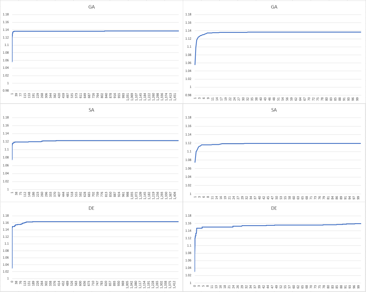
Here are the results for all three algorithms over the first 24 hours (left hand side) and the first 100 minutes (right hand side). As we can see, all algorithms get most of the way there in the first hour or two, but differential evolution outperforms both alternative optimization algorithms on this problem by a significant margin.

After this differential evolution was ran for a few more days, producing the following table:

// cache score
{0.f, 0.977f, 0.981f, 0.984f, 0.539f, 0.401f, 0.607f, 0.358f, 0.435f, 0.715f, 0.385f, 0.312f, 0.439f, 0.465f, 0.135f, 0.183f, 0.064f},
// valence score
{0.f, 0.944f, 0.678f, 0.417f, 0.434f, 0.481f, 0.322f, 0.297f, 0.271f},

This table is notably different from the vertex reuse table in that the first three elements are, in fact, close to 1. So the algorithm ranks the three vertices of the most recently seen triangle the highest.

As we discussed briefly earlier, this tends to result in a strip-like order. And indeed, this order happens to result in substantially smaller triangle strips as well - so it’s a great set of parameters to use when trying to reduce index count! However, the optimization was trying to minimize the size of compressed index data when ran through index encoder and deflate compression. The index encoder was designed to compress cache-optimized index sequences, not triangle-strip-like sequences - why is it doing better?

It turned out that the strip-like order has much more predictable triangle structure than a cache-optimized order. There’s a long sequence of triangles adjacent to one another that goes back and forth across the (topologically) planar areas of the mesh. This results in the index encoder generating more predictable encoded sequences⁹ which, in turn, results in deflate compressing the results better. The tuning algorithm picks up on that and finds the sequence that resembles strips without knowing anything about triangle strips - in fact, no part of the optimization pipeline knows about strips, they just happen to compress really well after the index codec!

But see, it gets even better. Once we know that triangle strips are an interesting target, it’s not too hard to slightly tweak the index codec to anticipate triangle strip-like input and produce even more efficient byte sequences on these. After which you can re-train the tables to minimize the size even further! Which is what I am doing as we speak¹⁰.

Conclusion

When this journey started, I viewed the vertex cache optimization algorithm as something that should be understood and tuned by a human. And this still seems very valuable and important - structural changes to the algorithm require a deep understanding of the problem.

However, studying the data is very powerful, and sometimes the machine can look for patterns on our behalf. This can be used to validate theories we have - it’s really fascinating to have the optimization process discover that something you thought to be true about the problem is, indeed, as far as we know, true! - and to discover theories we don’t yet have.

Optimization algorithms in particular are an incredibly effective tool to have in the toolbox. A lot of attention is on deep learning and study of differentiable programs these days, but even if you don’t know too much about how the target function behaves, and you can’t run the learning algorithm on a large cluster of GPUs, it’s still possible to leverage the data to come up with enlightening answers.