Voxel terrain: storage
27 Mar 2017It’s been about almost two years since we shipped the first version of smooth voxel terrain at Roblox, and with it being live for a while and seeing a lot of incremental improvements I wanted to write about the internals of the technology - this feature required implementing serialization, network replication, collision detection, ray casting, rendering and in-memory storage support and within each area some implementation details ended up being quite interesting. Today we’ll talk about voxel definition and storage.
What’s in a voxel?
Whenever you design a voxel system you have to answer a basic question - what defines a voxel? We wanted our terrain to implicitly define a mostly smooth surface with each point on the surface having a material value, so we could use some kind of contouring algorithm to generate polygons from the surface. Since it was important to have control over the surface in 3 dimensions (heightfield would not cut it), we needed to define the data that represents the surface. During a prototyping phase a few options became clear:
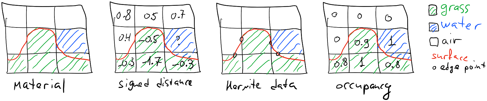
- Material. In this model we’d store just a material (an enum value) per voxel, and rely on neighboring voxels to construct the surface.
- Signed distance field. In this model we’d store the distance to the surface from the center of the voxel, with sign determining whether the center is outside or inside. This is a very well known model that’s frequently used to drive algorithms like Marching Cubes. We would also store the material per voxel.
- Hermite data. In this model instead of storing data about voxels, you store data about the intersections between surface and grid edges. Assuming the surface only intersects each voxel edge at most once, you have to store a bit for every edge that defines whether surface intersects this edge, an intersection point (which is defined by a 0..1 scalar), surface normal at the intersection point and the material at the vertices.
- Occupancy. In this model we’d store a material and the occupancy which defines the amount of matter around the voxel center - 0 meaning roughly that the voxel is completely empty and 1 meaning that the voxel is full.
We experimented with the material model and rejected it because it did not give us enough flexibility for tools - our voxels had to be pretty big for the solution to be practical for low end platforms, and thus we needed to be able to represent sub-voxel information (for example, to have a tool that can “erode” terrain on a scale much finer than a voxel size).
Hermite data was very interesting - you could build pretty rich tooling based on boolean operations and allow a fine control over smoothness of the surface. However, what wasn’t clear was how we would present this to developers in a form of API. We felt like CSG-based API such as “subtract a sphere out of terrain” was not sufficient - how do you implement a smoothing tool if this is all you have? - and we wanted to give our developers an API that allows full control over the terrain data such that you can implement any tool with it (in fact, all our existing terrain manipulation tools are using the public terrain API and are written in Lua). We didn’t feel like exposing raw Hermite data was an option due to its complexity so we had to discard this approach.
Signed distance field was more expressive than occupancy model, but ultimately resulted in similarly looking content and ended up having a more complicated mental model (how do I fill voxels that are far away from the surface? Does it even matter? How is the distance clamped? etc.) so we did not feel like it was worth the tradeoff.
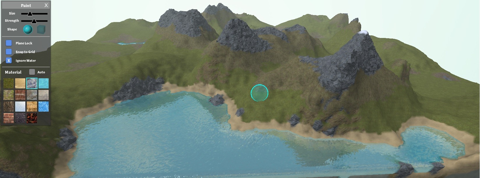
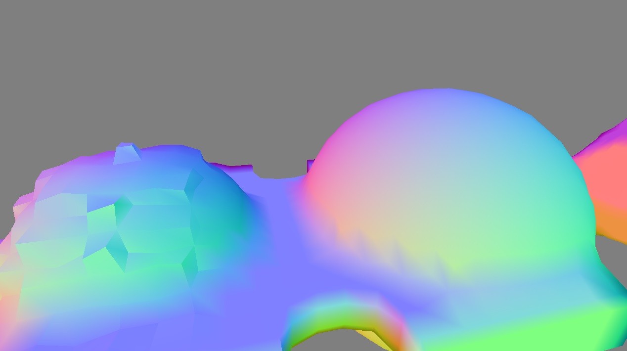
Thus we settled on the occupancy model, where every voxel would be defined by a material and occupancy pair. Our definition of occupancy is a bit peculiar because due to how our meshing algorithm works matter “overflows” from one voxel to another - occupancy 1 does not mean that the voxel looks like a cube, rather it just means that the voxel has as much matter as it can possibly contain. By discarding the Hermite model we lost an ability to precisely define sharp edges on the surface, which we decided to reclaim by using the material value - in addition to the texture that is applied the material also defines how terrain is shaped around the voxel; thus what defines geometry is the material and occupancy in the voxel and in voxel’s neighborhood. A screenshot from an early prototype shows how different materials with the same occupancy data can produce very different results:
Memory format
To represent a voxel, you need a material (which is an enum) and occupancy (which is a floating-point value in 0..1 range). Material storage is straightforward - we just store an index into the material table, which currently has 23 entries. To conserve space, we store occupancy as a quantized 8-bit value, which adds up to two bytes per voxel.
In a material-occupancy definition there is inherent ambiguity in terms of empty voxel representation - you can define it as occupancy = 0 but then the material choice does not matter; or you can define it as material = air but then the occupancy does not matter. We chose the model with an explicit Air material, and we decode occupancy as (value + 1) / 256.0 for non-air materials and 0.0 for air materials (which means that the occupancy is precisely represented in a floating point number which is not true for decoding methods like value / 255.0). Voxels with material = Air and occupancy != 0 are not valid; we make sure they never appear in the grid with simple branchless code:
// make sure occupancy is always 0 for Air material (0)
this->material = material;
this->occupancy = occupancy & (-static_cast<int>(material) >> 31);
When we originally developed the system, we decided to settle on a simple sparse storage format: all voxels would be stored in chunks 32x32x32 with each chunk represented as a linear 3D array (since each voxel needs two bytes for storage, this adds up to 64 KB per chunk; we also experimented with 16x16x16 chunks but the difference wasn’t very noticeable), and the entire voxel grid is simply a hash map, mapping the index of the chunk to the chunk contents itself:
HashMap<Vector3int32, Chunk> chunks;
It’s worth noting that we needed a sparse unbounded storage because our worlds do not have set size limits and you can use voxel content at any point; of course, voxel access in a local region needed to be very fast. A simple two-level storage scheme (hash map + 3D array) turned out to work really well for this - it’s simple to implement and reason about, and provides an easy way to trade “sparseness” for increased locality by adjusting chunk size. We ended up using this way of storing voxel data throughout the entire engine, with individual systems adjusting the chunk size to match the expected workload better (storage uses 32^3 chunks, network uses 16^3 chunks for initial replication and 4^3 chunks for updates, physics uses 8^3 chunks, rendering first used 32x16x32 chunks and later switched to chunks that increase in size from 16^3 up to 256^3 voxels).
Inside the chunk we ended up storing several 3D arrays - we call a 3D array of voxels “box” - of different sizes, forming a mipmap pyramid for our voxel content. We have 32^3 Box for the original content, and 16^3, 8^3 and 4^3 mipmaps that contain downsampled voxel data. The extra storage cost of mipmaps ends up being negligible, and the small penalty that we take for updating the mip levels when writing voxels to the voxel grid is well worth it considering that we are using them for Level Of Detail which allows us to render a lot fewer triangles in the distance, as well as for some other optimizations. The downsample algorithm that we use guarantees that if a voxel at a certain level of mip pyramid is filled with Air, all voxels corresponding to this area in the upper levels of the pyramid are also filled with Air - for example, if the bottom mip level has all 64 voxels empty then the entire chunk is empty.
Disk format
When it comes to storing voxels on disk, we wanted a more compact representation than a 3D array. There are a lot of ways to store voxels - we needed an encoding scheme that stored voxels as bytes (without any cross-byte bit packing to avoid efficiency loss of a byte-level lossless compressor - we usually take the encoded voxels and compress them further with LZ4), was reasonably efficient on the types of content we see frequently, and was simple - we could always upgrade the format later if we needed to spend more time doing it.
Our previous experiments in voxel technology suggested that if you take each chunk and do RLE compression on it, efficiently representing runs of voxels with the same contents, it resulted in pretty good compression rates and pretty efficient compression code. Remember, we don’t need to be optimal - we need to compress data to reduce it in size for storage efficiency, but we do frequently have a LZ codec running on top of that. Running RLE before LZ may seem counter-intuitive, but it significantly reduces the size of data making LZ faster, and in some cases means you don’t even need to do LZ compression because RLE on its own is enough - voxel data is frequently very regular.
An additional quirk is that each voxel in our system occupies two bytes; we wanted to have a more compact baseline representation so that even if RLE can’t find runs of sufficient length we still end up with a smaller file. A key realization is that many voxels are completely solid - if you imagine a mountain built from voxels, usually all interior voxels in the mountain only carry material information (that is still meaningful in case you want to dig a hole through the mountain later) - occupancy is usually 1 for these cells. Similarly, for Air we never need to store occupancy - it’s always zero! With this and RLE in mind, here’s the encoding we came up with:
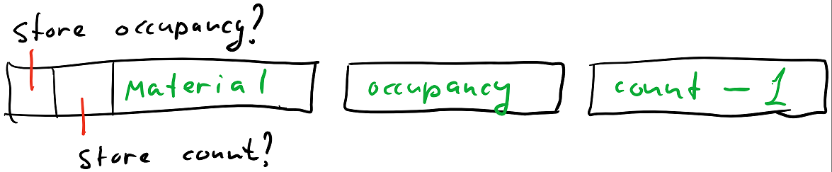
Each run of voxels starts with a byte that encodes the material (6 bits), whether we need to store the occupancy byte (1 bit) and whether we have a run length of more than one (1 bit). After this byte we store the occupancy value in a single byte (if the lead byte told us we needed it), followed by the run length in a single byte (if the lead byte told us we needed it). Since we encode single-voxel runs without a run length, we store run length minus one so that the longest run we can store is 256 voxels - we need to break up longer runs which is not a problem because you just need two bytes to encode a run as long as all voxels are solid or empty in case of Air.
Note that we only store count if we have more than one voxel in a run, so we could store
count-2instead ofcount-1; storingcount-1means that largest run is 256 voxels (which is a nice round number) and means we can use0later to extend the run format if necessary.
This encoding results in compression ratios close to 2x even without RLE, and with RLE it’s anywhere between 2x and 30x for real-world content; the maximum efficiency is reached for chunks that use just one material and all voxels are solid or empty; we can encode a chunk like this in 128 2-byte runs, which brings us from 64 KB per chunk to just 256 bytes (and a few bytes of metadata such as chunk index).
It’s definitely possible to improve on this encoding but this ended up working well for us. In addition to it serving as a file storage format, we also use it to compress undo history - whenever you perform an operation on the region of voxels, our undo system extracts the box of voxels from the grid before the operation, packs it using this encoding (the compression is extremely fast) and saves the result in case the user needs to undo the operation. We also use a variant of this with more aggressive bit packing and some other tweaks for network replication.
Memory format, take two
After we shipped the first version of our voxel system and started seeing a lot of adoption among developers, we started working on different ways to optimize the system in terms of both memory and performance. This was when we implemented rendering LOD which uses the mipmap levels and substantially reduces both time to render terrain and also memory required to store terrain geometry. After this optimization the bulk of memory cost of new terrain became the voxel data - storing two bytes per voxel just wasn’t going to cut it for low-end mobile devices.
At this point we had a lot of code written to assume that you can read a box of voxels from a terrain region and be able to iterate over the box very efficiently; some areas of the code went beyond reading a cell from a box one by one (which required two integer multiplications to compute the offset in a linear array) and used fast row access via a function like this:
const Cell* readRow(int y, int z) const;
We wanted to store voxel data more efficiently but we did not want to compromise on the access performance - we were willing to make voxel writes a bit slower, but voxel reads - which are required by every subsystem that works with voxel data - had to stay fast, and for some inner loops it was important to be able to quickly iterate through a row of voxels. In addition to the amount of effort to extract a voxel from the box memory locality was also crucial - we considered using some complicated tree structure but ultimately decided against it.
One obvious solution was to use our RLE scheme - keep chunks compressed in memory (either using pure RLE encoding or using LZ4 in addition to that), decompress on demand and keep a small cache of uncompressed chunks that are accessed frequently. This was a reasonable option but required to compromise on the read performance in case the chunk needed decompression - both LZ4 and our RLE decompressor are pretty fast but they are slower than just reading the memory, even after taking into account bandwidth savings. What we really wanted was a solution that allowed us to reduce chunk memory overhead but retain the read performance.
One of the issues was the chunk size. For some content 32^3 chunks weren’t imposing too much overhead, but for simple terrain that had almost no variation in height but was very large in XZ dimension the requirement to store 32 voxels along the Y axis for every non-empty chunk increased the memory overhead substantially. Terrains of such large sizes were previously impractical because of the lack of rendering LOD, but now rendering could handle this just fine if not for the voxel memory overhead. Reducing chunk sizes too much made read operations slower because read requests for large regions had to look up many chunks in the hash, and also increased the overhead of chunk metadata we had to store (for a 8^3 chunk the size of raw voxel data is just 1 KB so even a few pointers can add up to several percent of memory).
This is where we decided to use the ideas from our RLE packing to make a new in-memory compressed box representation. What worked well in RLE is packing each voxel in common cases into just one byte and assuming long contiguous runs of the same voxel data. If we now assume that these runs occupy full rows of data we can store chunks as follows:
- Each row (32^3 chunk has 32^2 rows) is either allocated or not.
- For unallocated rows, we store one byte - which represents the material value - and assume that all cells In this row are filled with this material and have “default” occupancy (1 for solid materials and 0 for air).
- For allocated rows, we store an offset into cell data, which is a linear array that contains data for all allocated rows in an uncompressed fashion.
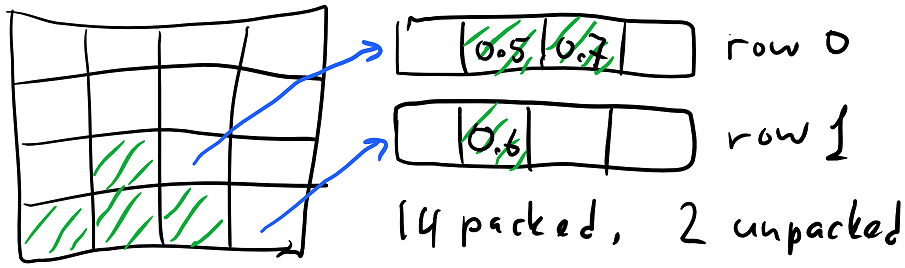
You can see how for a typical chunk (the diagram above shows a 4^3 chunk for simplicity), most rows will not be allocated - in this case 10 are empty and 4 are filled with grass with occupancy 1 - and the remaining rows, 2 in this case, need extra storage to specify material and occupancy for every cell.
In a 32^3 chunk we’d need up to 1024 allocated rows, which meant the row offset did not fit into one byte (it also doesn’t fit into one byte for 16^3 chunks because you need to dedicate some bits for the row state). There are some ways to work around the problem for 16^3 chunks but we decided to just use two bytes per row for the row header, which contains the “allocated” bit, and either the offset or the material value. To implement the function readRow, we have a global (read-only) array that contains pre-filled arrays of voxels for every material up to a certain chunk size, so we could implement the function like this:
const Cell* readRow(int y, int z) const
{
    uint16_t row = rows[y * size + z];

    return (row & kRowTagAllocated) ? rowdata + (row & kRowTagMask) * size : gCellRows[row & kRowTagMask];
}
Notice that this is constant-time and also very very fast - the voxel read performance did not suffer as a result of this change (and instead improved since we need to read less memory).
Writing becomes more complicated because we sometimes need to write cells into unallocated rows, which requires reallocating the cell content - we split the write workloads into two stages where the first stage marks the rows that will be written to, then we reallocate the chunk if necessary, and then actually perform the writes of new cell data. When we mark the rows we analyze the content we’re going to write there to keep the rows packed (unallocated) if possible. This resulted in code that was slower and more complicated, but voxel writes are relatively rare. There are some artificial cases in our scheme where repeatedly doing tiny writes can repack the chunk too many times - this is pretty simple to work around though because you can always pessimistically unpack the entire chunk at any point by allocating all rows.
The worst case impact of this change is that we spend 2 bytes for every row in addition to whatever we had before, which adds 2 KB to a 64 KB chunk; most chunks have at least several rows compressed, and in some levels the impact is quite dramatic - for an extreme example, a layer of voxels that is just one voxel thick in Y dimension will have all rows unallocated which turns 64 KB chunks into 2 KB, reducing memory impact 32x. Of course the memory savings vary depending on the content - one nice side effect of this change is that the chunk size impacts memory much less because the packed representation does not spend extra memory for empty rows.
Results and future work
To give you some idea of the resulting sizes, these numbers were captured on a very large procedurally generated level with many biomes using different materials, with mountains, cliffs, canyons and caves; this level has about 1 billion non-empty voxels:
| Storage | Size | Bytes per voxel |
|---|---|---|
| Disk (RLE) | 73 MB | 0.07 |
| Disk (RLE+LZ4) | 50 MB | 0.05 |
| Disk (RLE+zstd) | 38 MB | 0.04 |
| Network (bit-packed RLE) | 59 MB | 0.06 |
| Memory #1 (unpacked) | 2973 MB | 2.97 |
| Memory #2 (row packed) | 488 MB | 0.49 |
Clearly RLE is very efficient at compressing this data; we do get further improvements using LZ4 but they are not very substantial, and the more valuable option is to employ entropy coding. What also works very well is using RLE and packing data a bit more tightly - this has an advantage that it compresses and decompresses data very quickly and requires no state so it works well for network packets where we only need to send a small chunk, although using byte packed RLE with a fast general compressor on top of it would also work well.
Also note that, while with a naive chunked storage format we need more than 2 bytes per voxel to store data in memory with fast access (2 bytes per voxel would be optimal, but this is where the chunk size comes into play - the bigger the chunks are, the more memory you waste on empty voxels), our new row packed format reduces it by a factor of 6, which gives us 0.5 bytes per voxel and preserves very fast random access and linear read performance.
None of the methods presented above are very complicated, but this is pretty much the point - the simpler the code that we ship ends up being, the easier it is to reason about its performance and behavior, and the easier it is to rework it later. Ultimately while there are ways to compress data better, and probably also ways to organize data for faster access, what we ended up with has a nice balance between performance, simplicity and compactness and solved the issues we had - compared to the raw storage, storing undo data as RLE compressed chunks and voxel data as row-packed chunks is significantly more efficient and does not have a noticeable performance impact on our workloads.
We are pretty happy with the resulting solution; one thing to improve is that we currently send baseline mip level over the network, which means that for big levels it takes a lot of bandwidth to send data that’s so far away that rendering will not use the baseline mip for it anyway. Since we already have the mip data it makes a lot of sense to send it instead - which we haven’t done yet but definitely will do in the future. This mostly requires careful management of data that the client has or doesn’t have, and requires limiting the physics simulation to only work in the regions where we have the full resolution data, because our physics code uses it to generate collision data - which will be the topic for a following post.
| « Metal retrospective | Optimal grid rendering isn't optimal » |