Efficient jagged arrays

A data structure that comes up fairly often when working with graphs or graph-like structure is a jagged array, or array-of-arrays. It’s very simple to build it out of standard containers but that’s often a poor choice for performance; in this post we’ll talk about a simple representation/construction code that I found useful across multiple different projects and domains.

Crucially, we will focus on immutable structures - ones that you can build in one go from source data and then continuously query without having to change it. This seems like a major constraint but for many problems it is sufficient to build the structure once, and it makes significantly simpler and more efficient implementations possible.

Applications

Graphs seem like an abstract data structure out of a CS graduate course, but they come up fairly often in diverse algorithms. Here are a few examples for why you might want to use a jagged array:

• For mesh processing, given an index buffer, it would be useful to build a list of triangles that each vertex belongs to
• For other mesh processing algorithms, instead of triangles you might want to keep track of edges that each vertex belongs to
• For intermediate representations in a compiler, you might want to build a list of basic blocks that jump to a given basic block (aka predecessors)
• For transform graphs where every node only specifies a parent node, you might want to build a list of children for every node

In all of these examples, you’re starting from a set of data that already contains the relevant relationship (parent-child, vertex-triangle), but for efficiency creating a data structure that can be used to quickly look up the entire set is useful. For example, to compute an average vertex normal, you’d need to aggregate triangle normals from all incident triangles; there are ways to do this without building adjacency structures but if crease handling is desired, it can be difficult to incorporate into an algorithm if adjacency is not available.

In all cases above, the immutability is often tolerable. For example, the mesh topology might be static throughout the algorithm, or the basic block information might only change infrequently and as such can be recomputed on demand.

Naive implementation

For concreteness, we will assume that we’re building a triangle adjacency structure, where for each vertex we need to keep track of all triangles it belongs to. Given the index buffer and number of vertices, the solution is very simple¹:

std::vector<std::vector<unsigned int>> adjacency(vertex_count);

for (size_t i = 0; i < index_count; ++i)
{
    unsigned int triangle = unsigned(i / 3);

    adjacency[indices[i]].push_back(triangle);
}

The code is simple but has a number of efficiency problems²:

• For each vertex we’re paying an overhead of sizeof(std::vector), which is 24 bytes on a 64-bit system, just to store the array - even if the vertex is not used. This is a memory problem as well as a performance problem since lookups into adjacency will use more cache space than necessary.
• Because std::vector grows exponentially, typically with a factor of 1.5, we might also lose memory on the extra elements that never end up being used. If the length of each list is 6 on average, the vector capacity will be 8, losing ~8 bytes per vertex.
• Because std::vector stores data on heap, we will end up also potentially wasting memory on allocation metadata and block rounding. The size depends on the allocator, on Linux we end up wasting ~16 bytes between each allocation to allocation headers.
• In addition, we will need to reallocate each vector continuously as we’re pushing new elements. The growth of std::vector is particularly slow for small sizes, and to get to size 6 we will need 4 allocations. This results in a substantial performance overhead, as doing this many small allocations and deallocations could easily dominate the performance of the algorithm. While this (and the previous) problem can be mitigated by reserving the size of each element up-front if we have a guess³, if our guess is off in either direction we could waste more memory or more time.

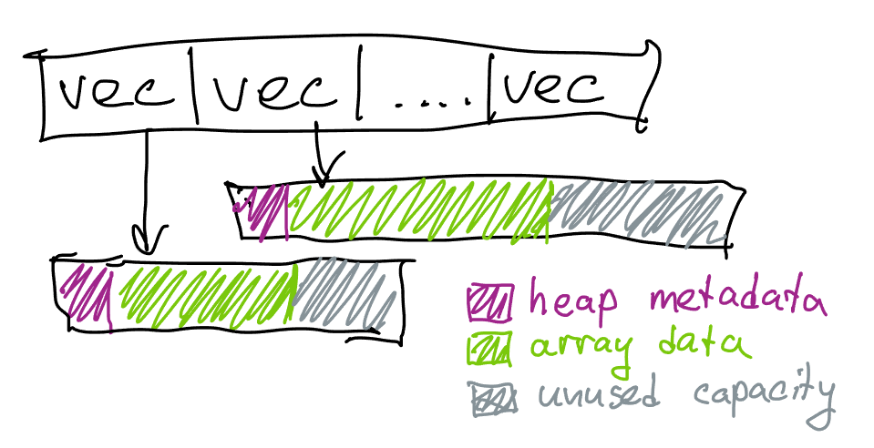
For code above if each vertex belongs to 6 triangles, the allocations where the actual lists are stored are going to be ~48 bytes apart on Linux; this is reasonable from the macro locality perspective⁴, but given that we only have ~24 bytes of data (6 * sizeof(unsigned int)) it still means that traversing this data would waste ~half of the bytes loaded into cache, even ignoring the sizeof(std::vector) (which is also 24 bytes, so in total we’re using ~72 bytes per vertex to store just 24 bytes of triangle indices).

Counting once

The majority of inefficiencies all come from the fact that we aren’t quite sure how long each per-vertex list of triangles should be; guessing this number up front can misfire, but given that the lists are not going to change in size after the adjacency computation is done, we can do much better by counting the list sizes first in a separate pass. Once that’s done, we will be able to reserve each vector to the exact size that it needs, and fill the lists as we did before.

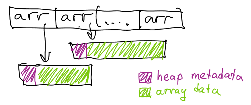
While we are here, we can also replace std::vector with a plain old array pointer that we allocate with new - after all, we’re paying a substantial memory cost for each std::vector object since it needs to manage the size and capacity fields.

struct Triangles
{
    unsigned int count = 0;
    unsigned int offset = 0;
    unsigned int* data = nullptr;
};

std::vector<Triangles> adjacency(vertex_count);

for (size_t i = 0; i < index_count; ++i)
    adjacency[indices[i]].count++;

for (size_t i = 0; i < vertex_count; ++i)
    if (adjacency[i].count > 0)
        adjacency[i].data = new unsigned int[adjacency[i].count];

for (size_t i = 0; i < index_count; ++i)
{
    unsigned int triangle = unsigned(i / 3);

    adjacency[indices[i]].data[adjacency[indices[i]].offset] = triangle;
    adjacency[indices[i]].offset++;
}

We now need to do one more pass through the source data to compute the size of each individual list; once that’s done, we can allocate the exact number of entries and fill them with a second pass. While we’re here, we can also use 32-bit integers instead of 64-bit integers for count and offset, unless we want to process vertices that are part of >4B triangles.

Let’s see how we’re doing on our efficiency goals.

• Instead of ~4 allocations per vertex, we now use just one, immediately allocating the array of correct size
• We’re using less memory per vertex because we aren’t using std::vector anymore; sizeof(Triangle) is only 16 bytes.
• We’re still losing memory on allocation metadata and block rounding; on Linux, we end up only using ~32 bytes of memory for each allocated block though.

In total, we’ve reduced the total number of allocations to one per vertex, and the total amount of memory per vertex from 72 bytes to 48 bytes. Naturally, we can do better.

Merging allocations

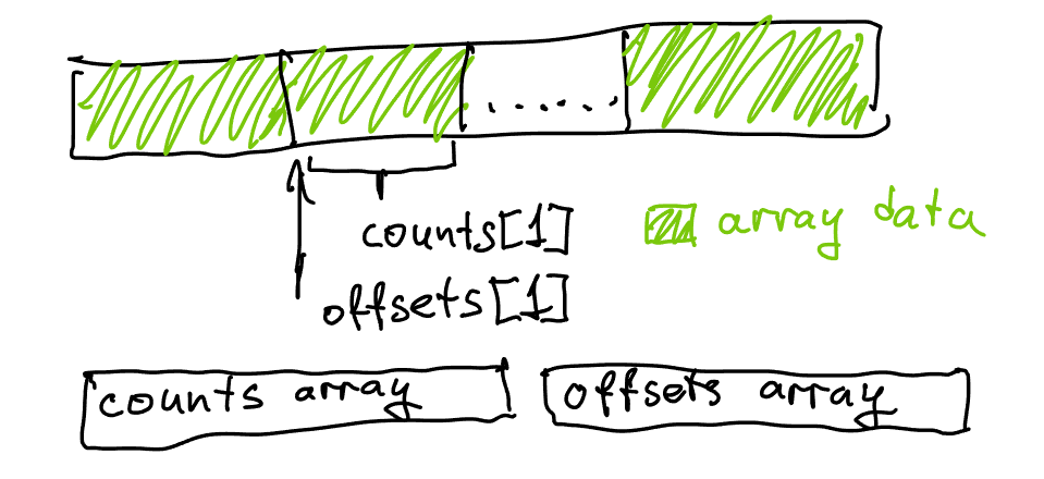
The major source of remaining inefficiencies is the fact that each list is allocated separately. A much more efficient approach would be to allocate enough memory for all the lists and then place each list at an offset in the resulting large allocation such that for each list, the items of that list follow the items of the list before it. This sounds as if it would require a lot of extra code and tracking data, but it turns out we are in a reasonable position to do this without too much extra complexity:

Note that in our previous solution, just precomputing count was not enough: we also needed to track offset for each vertex during the algorithm’s operation, as we needed to know which element in each triangle list to write to next. With one more pass over the counts, we can instead compute the offset assuming all lists are in one large allocation: instead of each offset starting from 0, we will start offset for each vertex with the total number of elements needed by all preceding vertices. This will allow us to allocate all triangle lists as part of one large allocation, and stop storing the pointer to each list in each vertex. The initial value for each offset is known as a prefix sum and is trivial to compute in one pass.

After we do that and fill all lists, we will have shifted each offset by the size of each list - in order to refer back to the correct range, we will need to subtract count from offset again to compensate for the extra additions. This was not a problem in our previous solution because we’d store a pointer in each list, but now that all the memory for all lists is shared we need offset to refer to the contents of each list when actually using the adjacency structure.

struct Triangles
{
    unsigned int count = 0;
    unsigned int offset = 0;
};

std::vector<Triangles> adjacency(vertex_count);

for (size_t i = 0; i < index_count; ++i)
    adjacency[indices[i]].count++;

unsigned int sum = 0;

for (size_t i = 0; i < vertex_count; ++i)
{
    adjacency[i].offset = sum;
    sum += adjacency[i].count;
}

std::vector<unsigned int> data(sum);

for (size_t i = 0; i < index_count; ++i)
{
    unsigned int triangle = unsigned(i / 3);

    data[adjacency[indices[i]].offset] = triangle;
    adjacency[indices[i]].offset++;
}

// this corrects for offset++ from the previous loop:
// use &data[adjacency[vertex].offset] when querying adjacency
for (size_t i = 0; i < vertex_count; ++i)
    adjacency[i].offset -= adjacency[i].count;

Instead of allocating each list separately we now put them all one after each other in a large allocation. This packs the data more densely and allows us to use indices instead of pointers to refer to individual elements, as well as eliminating all allocation waste and overhead.

Note that in the code above, offset is now tracking a “global” offset - which is to say, we now expect that the sum of all lengths of all lists fits into a 32-bit integer. This is valuable for memory efficiency, but does technically restrict this structure to slightly smaller data sources. It’s easy to change by using size_t for offset and sum if necessary.

Let’s see how we’re doing on our efficiency goals.

• We are now using 0 allocations per vertex (2 allocations total).
• Each vertex needs 8 bytes of data for maintaining the list (count and offset)
• The lists themselves are stored tightly without any extra memory overhead

Each vertex is now thus using 8+24 = 32 bytes of memory (assuming an average list length is 6), which is fairly close to optimal… but we’re not quite done yet.

Removing counts

Up until this things were mostly pretty intuitive; I’ve used data structures computed in a similar manner to above for years. Recently I’ve realized there’s still a little bit of redundancy left and I totally did not just spend writing this entire post to mention this one tiny tweak, which is probably also widely used elsewhere, to an otherwise standard construction.

Consider an array of counts, [1 6 5 3 6] for example, that we’ve computed in the first loop.

Our second loop computes a running sum, filling offsets with [0 1 7 12 15], and yielding sum=21. These are the offsets where each individual list will live.

Our third loop actually fills all the list items, and in doing so advances each offset to get to the following offsets array: [1 7 12 15 21].

Our fourth loop finally corrects this by subtracting count from each element.

If you look at the shifted offset array carefully, it’s actually almost a subset of our initial offsets array! Which really makes sense: if offsets[v] is initially pointing at the beginning of each individual list, then after we filled all the lists offsets[v] is pointing at the end of the list - which also happens to be the beginning of the next list due to how we’ve laid out all lists in memory!

This means that we don’t need to adjust the offsets using counts - we can simply shift the elements forward by 1 in the array – conceptually. Or we can simply fill the elements in the right place in the array. This also means that counts, once filled in the initial loop and used in the prefix sum, are no longer necessary - except in iteration when querying adjacency lists, but there we can simply use offsets[v + 1] to denote the end of the range where the list is stored.

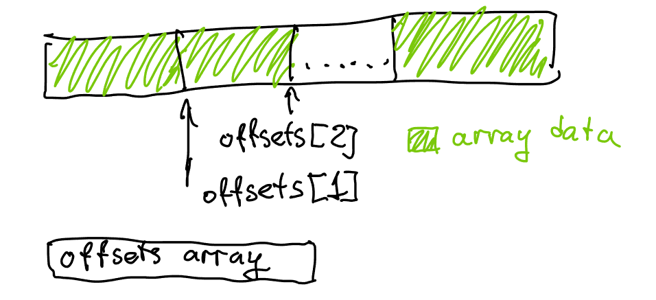
This allows us to mostly ignore count - we still need to compute it once, but we’ll store it in the offsets[] array, and all further operations will work with offsets. Instead of shifting the array by moving the elements around, we will simply carefully adjust the offset indexing, which will save us the trouble of doing any offset correction at the end.

// note: we allocate one extra element so that when querying, we use:
// &data[offsets[v]] .. &data[offsets[v + 1]]
std::vector<unsigned int> offsets(vertex_count + 1);

// offsets[0] starts at 0 and stays 0
unsigned int* offsets1 = &offsets[1];

// compute count into offsets1
for (size_t i = 0; i < index_count; ++i)
    offsets1[indices[i]]++;

// transform counts into offsets in place
unsigned int sum = 0;

for (size_t i = 0; i < vertex_count; ++i)
{
    unsigned int count = offsets1[i];
    offsets1[i] = sum;
    sum += count;
}

// populate lists; this automatically adjusts offsets to final value
std::vector<unsigned int> data(sum);

for (size_t i = 0; i < index_count; ++i)
{
    unsigned int triangle = unsigned(i / 3);

    data[offsets1[indices[i]]] = triangle;
    offsets1[indices[i]]++;
}

// all done!

Compared to our previous solution, we no longer need a final loop to correct the data, but more importantly we don’t need to explicitly track count anymore which saves us ~4 bytes per vertex and yields a fairly optimal⁵ general solution. Note that you can still replace unsigned int with size_t for offsets if the total number of elements can ever exceed 4B, which would still only use 8 bytes per vertex for metadata.

To iterate through the resulting structure, offsets and data need to be retained as they compose the entirety of the data structure (offsets1 is temporary and just simplifies the code a little bit):

const unsigned int* begin = &data[offsets[vertex]];
const unsigned int* end = &data[offsets[vertex + 1]];

for (unsigned int* tri = begin; tri != end; ++tri)
    // do something with the triangle index

Conclusion

The jagged array in a single allocation (or two) is surprisingly useful and versatile! Hopefully you’ve liked the post, which I tried to structure such that transformations from naive to optimal solution are intuitive and have a clear rationale. There are other algorithms and data structures that can benefit from similar optimizations; most crucially, cleanly splitting the operations into “build” and “query” such that you can build up the structure in one go is something that can be used in many other cases to get to a much better data layout or performance, whether driven by algorithmic complexity or machine efficiency. Past which, it really pays off to be careful with allocations and structure as much data as possible in the form of large directly indexable arrays.

Note: After publishing this, Paul Lalonde on Mastodon noted that the final algorithm can be a good match for GPU processing: between atomics for the counting/filling phase, and a plethora of fast parallel prefix sum algorithms, the construction of this data structure can be done entirely on the GPU with a few compute shaders/kernels, and once built the structure is easy and fast to query as well.

Sometimes, ability to mutate is still important and some ideas from this post will not apply. Some algorithms in meshoptimizer use the second-to-last variant of the code (with counts and offsets separated): while it does not allow for arbitrary mutation, it does allow removing elements from the individual lists which can speed up the adjacency queries in some cases, so merging these two is not always fruitful.