Approximating slerp

Quaternions should probably be your first choice as far as representing rotations goes. They take less space than matrices (this is important since programs are increasingly more memory bound); they’re similar in terms of performance of basic operations (slower for some, faster for others); they are much faster to normalize which is frequently necessary to combat accumulating error; and finally they’re way easier to interpolate. In this post we’ll focus on interpolation.

If you’ve read “Hacking Quaternions” (2002) by Jonathan Blow, then this article will be familiar. Then again, it’s been 13 years, and these results are more precise and more rigorously derived.

Spherical interpolation

A well known method of interpolating quaternions is called $slerp$ or spherical interpolation. Spherical interpolation is a linear combination of two quaternions with the coefficients that depend on the half-angle of rotation between the quaternions:

$ a = \arccos(q_0 \cdot q_1) $

The most important feature of $slerp$ is that the interpolation has constant angular velocity - that is, the angle of rotation from $q_0$ to the resulting quaternion changes as a linear function of interpolating coefficient $t$. $slerp$ is defined as follows:

$ slerp(q_0, q_1, t) = q_0\frac{\sin((1 - t) a)}{\sin(a)} + q_1\frac{\sin(t a)}{\sin(a)} $

This function has a singularity at $a = 0$ (which corresponds to $q_0 = q_1$), so in practice $slerp$ is replaced by a simple linear interpolation as $q_0$ approaches $q_1$. In addition, because of quaternion double-cover - for each rotation there are two unit quaternions that represent it, $q$ and $-q$ - $slerp$ implementation has to account for that and negate one of the quaternions if $q_0 \cdot q_1$ is negative.

The problem with $slerp$ is that it’s expensive to compute. You have to evaluate four trigonometric functions; since they are usually implemented using a range reduction step followed by a polynomial approximation with a relatively high power, this can get expensive. We can try to replace them with simpler approximations that are less precise, but it’s more efficient to solve this issue in a more direct way.

One other way to interpolate quaternions is $nlerp$ - which is just a linear interpolation, followed by a renormalization step (as well as aforementioned negation to solve issues with double-cover). Here’s how it can work:

Q nlerp(Q l, Q r, float t)
{
	float lt = 1 - t;
	float rt = dot(l, r) > 0 ? t : -t;

	return unit(lerp(l, r, lt, rt));
}

This code assumes that unit normalizes the quaternion and lerp performs the computation l * lt + r * rt.

This is much simpler than $slerp$ - the only semi-expensive step here is normalization (but even this is pretty efficient given the reciprocal square root intrinsics that are present in most SIMD instruction sets). However, this does not give us constant velocity interpolation.

Despite not having constant velocity, $nlerp$ follows the same path as $slerp$ - both operations produce values that lie on the shortest arc between the two input quaternions. This naturally means that by adjusting the coefficient of interpolation in $nlerp$ we can get the same result as computed by $slerp$.

For many applications constant velocity is not actually very important - for example, if you use quaternions in your animation system, it’s possible that your artists made the animations using spline-based Euler angle interpolation. So the choice of the interpolation is to an extent arbitrary - the canonical way of exporting animations is starting with a high-frequency sampled animation (e.g. 60 Hz), and removing keyframes while the interpolation error is acceptable. If this is the case, a different interpolation method will just change the number of keyframes so maintaining constant velocity is not critical. For the rest of the article though we will assume that we need a close-to-constant angular velocity interpolation.

Approximating slerp with nlerp

This is the equation we’re solving (we need to find $t'$):

$ nlerp(q_0, q_1, t') = slerp(q_0, q_1, t) $

Given that, and some normalizing factor $s$ (remember, nlerp is a linear interpolation followed by normalization), we have:

$ \frac{q_0(1 - t') + q_1 t'}{s} = q_0\frac{\sin((1 - t) a)}{\sin(a)} + q_1\frac{\sin(t a)}{\sin(a)} $

Let’s assume that the coefficients of linear combination are equal (if they are the equality will surely hold); from that we get:

$ s' = \frac{s}{\sin(a)} $

$ \frac{1 - t'}{s'} = \sin((1 - t) a) $

$ \frac{t'}{s'} = \sin(t a) $

From that it’s easy to get $t'$:

$ \frac{1}{s'} = \frac{1 - t'}{s'} + \frac{t'}{s'} = \sin((1 - t) a) + \sin(t a) $

$ \frac{1}{t'} = \frac{1 / {s'}}{t' / {s'}} = \frac{\sin((1 - t) a) + \sin(t a)}{\sin(t a)} $

$ \frac{1}{t'} = 1 + \frac{\sin((1 - t) a)}{\sin(t a)} $

$ t' = \frac{1}{1 + \frac{\sin((1 - t) a)}{\sin(t a)}} $

This derivation leads us to the final formula that uses the cosine of the angle between quaternions as the parameter $d$:

$ d = q_0 \cdot q_1 $

$ t' = \frac{1}{1 + \frac{\sin((1 - t) \arccos d)}{\sin(t \arccos d)}} $

Now that we know how to compute $t'$, we need to find a good approximation that is fast to compute - which means a polynomial approximation. Note that we need to compute $d$ anyway to determine if we need to flip one of the quaternions - so if we can efficiently approximate $t'$, we can get an interpolation function that’s as precise as $slerp$ and as fast as $nlerp$!¹

The first step to finding a good approximation is looking at the data - in this case, at the function $t' = t'(d, t)$².

Staring at the data

The easiest way to analyze the function is to graph it over the domain we’re interested in. Let’s first visualize our function in 3D over $[0..1]$:

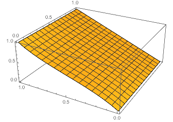
$t'(d, t)$

This looks close to a plane, suggesting that $t'(d, t) \approx t$. Thus the difference will probably be easier to look at:

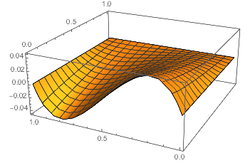
$t'(d, t) - t$

This looks interesting - our function seems to resemble a cubic polynomial in any d-slice. Let’s plot several 2D slices at different values of d:

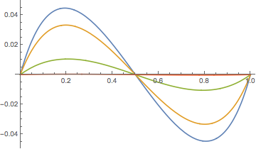
$t'(d, t) - t,\space d=0.01, 0.2, 0.7, 0.99$

Every d-slice of our function has three roots - 0, 0.5, 1. In these values the value of $t'$ is the same as $t$, which means that $nlerp$ is exact in these three points³. This also suggests that a polynomial approximation of $t'(d, t) - t$ has $t(t-0.5)(t-1)$ as factors. The simplest approximation is thus $t'(d, t) \approx K(d)(t-1)(t-0.5)t+t$, where $K$ is the factor that “flattens” the spline as seen on the graphs.

Is this a good approximation? Let’s check!

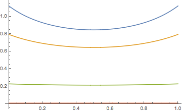
$K(d, t)=\frac{t'(d, t) - t}{t(t-0.5)(t-1)},\space d=0.01, 0.2, 0.7, 0.99$

From this it is obvious that while $K$ is reasonably flat, for small values of $d$ that correspond to large angles between input quaternions it resembles a quadratic polynomial of the form $A(t-0.5)^2+B$ (the form is apparent because lowest point is at $t=0.5$). We now know that we can either model $K(d, t)$ without taking $t$ into account, which will give results that are less accurate, or model $K(d, t)$ as a quadratic polynomial with coefficients that depend on $d$ alone.

Let’s explore both options.

Fitting K(d)

For any values of $d$ and $t$, we can compute $K(d, t)$. If we model $K$ as a value that does not depend on $t$, this gives us a lot of points that conflict - e.g. for a given value of $d$ we’d want $K$ to take a set of different values. You can think of this as having a lot of points on a plane and trying to fit them to a function. It makes sense to first plot these points, which is what we will do:

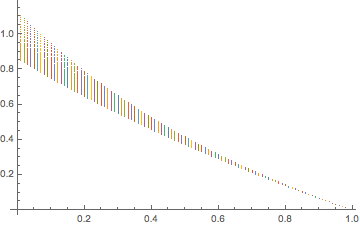
$K(d, t)$

This looks like a quadratic polynomial. Of course since this is not a function any approximation will give an error - we can find a polynomial that minimizes the sum of squares of the errors using least squares fitting, which yields our result:

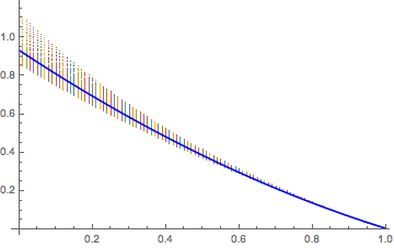
$0.931872 - 1.25654 d + 0.331442 d^2$

Thus our first approximation becomes:

$ K_0(d, t) = 0.931872 - 1.25654 d + 0.331442 d^2 $

Fitting K(d, t)

To get a more precise approximation, we’ll have to find $A$ and $B$ in $K(d, t) = A(t-0.5)^2+B$. $K$ has a singularity at $t=0.5$, but we can evaluate it at $t=0.49$ to get an estimate of $B$, and evaluating at $t=0.01$ gets us $0.25A+B$. Both values will depend on $d$ so naturally we will plot them:

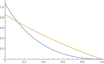
$A=4*(K(d, 0.01)-K(d, 0.49)),\space B=K(d, 0.49)$

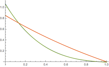
The blue line represents $A$ and looks like a parabola; the orange line represents $B$ and looks like a line. Let’s first try to fit both of them independently:

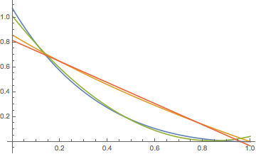
$A=4*(K(d, 0.01)-K(d, 0.49)),\space B=K(d, 0.49),\space A' \in P_2,\space B' \in P_1$

The fit is not very good - it looks like we’re missing an extra degree in both polynomials. Let’s try to approximate $A$ using a cubic polynomial and $B$ using a quadratic one:

$A=4*(K(d, 0.01)-K(d, 0.49)),\space B=K(d, 0.49),\space A' \in P_3,\space B' \in P_2$

This is much better. The resulting polynomials that we get are:

$ A_1(d) = 1.0615 - 2.97792 d + 2.89199 d^2 - 0.983735 d^3 $

$ B_1(d) = 0.853322 - 1.07504 d + 0.225676 d^2 $

$ K_1(d, t) = A_1(d)(t-0.5)^2 + B_1(d) $

One issue is that we were fitting the polynomials $A$ and $B$ independently, and we were assuming that $K(d)$ is a quadratic polynomial, which is just an approximation. The errors from multiple approximations that we fit independently will accumulate and we won’t get the best results. Since we know the final form we want, we can fit the entire expression at once - Mathematica can do this using FindFit function (and black magic). This gives us the following result:

$ A_2(d) = 1.0904 - 3.2452 d + 3.55645 d^2 - 1.43519 d^3 $

$ B_2(d) = 0.848013 - 1.06021 d + 0.215638 d^2 $

$ K_2(d, t) = A_2(d)(t-0.5)^2 + B_2(d) $

Evaluating approximation error

All of the approximations we computed above were using least-squares error metric in terms of $K$. However, $K$ is not really meaningful since this is just an intermediate value necessary to compute $t$. We can compute the error in $t$ but the ultimate metric that we care about is the interpolation result - how much does the resulting quaternion deviate from the one obtained using $slerp$?

Without loss of generality we can assume that the input quaternions were $q_1=(0,0,0,1)$ and $q_2=(\sqrt{1-d^2},0,0,d)$. The scalar component of the result of $nlerp$ is thus:

$ q_{lerp} = (\sqrt{1-d^2}t',0,0,(1-t')+dt') $

$ q_{nlerp} = \frac{(\sqrt{1-d^2}t',0,0,(1-t')+dt')}{|(\sqrt{1-d^2}t',0,0,(1-t')+dt')|} $

$ q_w = \frac{(1-t')+dt'}{\sqrt{(1-d^2){t'}^2 + (1-t'+dt')^2}} $

Since the scalar component of the quaternion is the cosine of the half-angle of rotation, and in our case we’re starting from angle 0, we expect that for any parameter $t$ we’ll get the half-angle $t\arccos d$. This lets us define the absolute angular error:

$ e = 2|t\arccos d - \arccos \frac{(1-t')+dt'}{\sqrt{(1-d^2){t'}^2 + (1-t'+dt')^2}}| $

We can now measure the maximum error for $nlerp$ and all three representations and get:

$ e_{nlerp} = 1.42229 * 10^{-1} = 8.15^{\circ} $

$ K_0: e_0 = 6.96632 * 10^{-3} = 0.40^{\circ} $

$ K_1: e_1 = 1.09562 * 10^{-3} = 0.06^{\circ} $

$ K_2: e_2 = 7.76255 * 10^{-4} = 0.04^{\circ} $

This is pretty good - remember, this is the maximum absolute error across our entire range! We can clearly see that our efforts to make the approximation more precise paid off - using a more involved approximation for $K$ together as well as carefully fitting the coefficients reduced the error by an order of magnitude. Also note that all errors reach their maximum value for quaternions that are at almost $180^{\circ}$ rotation from each other. If we reduce the interval so that initial quaternions are at most $90^{\circ}$ from each other, we get:

$ e_{nlerp} = 1.60363 * 10^{-2} = 0.91^{\circ} $

$ K_0: e_0 = 1.12533 * 10^{-4} = 0.006^{\circ} $

$ K_1: e_1 = 1.24728 * 10^{-4} = 0.007^{\circ} $

$ K_2: e_2 = 7.22881 * 10^{-5} = 0.004^{\circ} $

It’s interesting that while our approximations do help, they are not that different from each other once the angle between the quaternions is not too high. This makes sense if you recall that $K$ was very flat for large values of $d$ - so we don’t really get more precision because our basic approximation was good enough!

Note also how we got pretty good results despite the fact that we did not optimize for the maximum error. All of the fits that we did minimized the sum of squares of the errors; additionally, our error was not in terms of the angle but in terms of some internal parameters. I tried to explicitly refit the equations to minimize the maximum angular error, but was not very successful - the results ended up being close so let’s leave it at that.

Now that we got two good approximations and analyzed the error we can make an informed decision of whether to use a more or less precise implementation. In the next article we will look at the implementation of proposed approximations to see the relative performance of all interpolation methods.