Billions of triangles in minutes

Early this year, NVIDIA released their new raytracing technology, RTX Mega Geometry, alongside an impressive Zorah demo. This demo was distributed as a ~100 GB Unreal Engine scene - that can only be opened in a special branch of Unreal Engine, NvRTX. The demo showcased the application of new driver-exposed raytracing features, specifically clustered raytracing, in combination with Nanite clustered LOD pipeline - allowing to stream and display a very highly detailed scene with full raytracing without using the Nanite proxy meshes that Unreal Engine currently generates for raytracing.

As this was too Unreal Engine specific for me, I couldn’t really experiment much with this - but then, in early September, NVIDIA released an update to their vk_lod_clusters open-source sample, that - among other things - featured Zorah scene as a glTF file. Naturally, this piqued my curiosity - and led me to spend a fair amount of time to improve support for hierarchical clustered LOD in meshoptimizer.

Technology

The rest of this will be easier to understand if you have a reasonable grasp of Nanite. If not, I highly recommend Nanite: A Deep Dive by Brian Karis et al which talks about the specifics; I’ll just summarize the basic flow here.

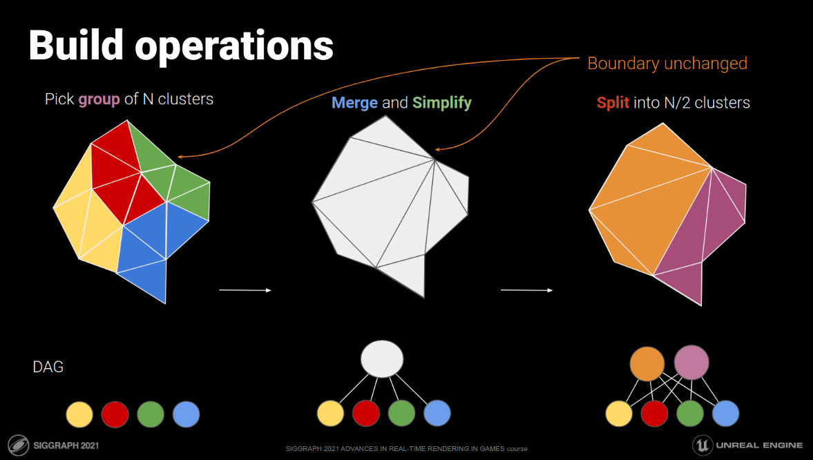
Given a triangle mesh with, probably, a lot of triangles, our task is to 1) generate a hierarchical structure that can represent this mesh at any level of detail, 2) stream parts of this structure at appropriate detail, and 3) render the visible parts of the mesh at appropriate detail level. It’s important that the structure we use can represent multiple levels of detail in multiple different regions of the mesh - this allows it to scale to large models while distributing the detail appropriately; it’s also important that it is efficient to render. The structure that’s chosen here is a graph (DAG) of clusters; each cluster is a small set of triangles, say, up to 128, and represents a small patch of the mesh at a given level of detail. The structure contains clusters at various levels of detail, and the runtime code is responsible for streaming and rendering them to minimize the visual error - a cluster is replaced by a coarser cluster only if the resulting visual error is under 1 pixel (and the resulting switch is hidden by TAA or other temporal filters).

There are three tricky parts to this technique: generation of the structure from the highly detailed mesh; compression of the results to make them efficient to stream; and real-time rendering of the results. We are only going to talk a little bit about the first part :)

To build the structure, a mesh is split into a set of clusters; neighboring clusters are merged in slightly larger groups; each group is simplified independently, preserving the boundary edges of the group; the resulting group is then split into more clusters and the process recurses until no admissible clusters are left. There is a lot of nuance in how the algorithms are combined to ensure that the resulting representation doesn’t exhibit cracks between clusters at various levels of details, and a lot of tradeoffs for individual algorithms involved - easily the subject of a thesis (and indeed, multiple theses have been written on this topic).

Since Nanite was released in 2021, multiple different engines started adopting this processing paradigm. An open-source geometry processing library I work on these days, meshoptimizer, since 2024 has had an example of how to combine multiple different algorithms that meshoptimizer provides to build the resulting structure¹. Having an end-to-end example made it much easier to improve the algorithms and experiment with variants of the higher level technique - could I perhaps use that example code to process the Zorah scene?

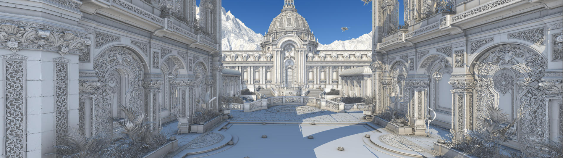
A sense of scale

That screenshot above certainly looks pretty; getting to that level of fidelity requires a lot of texture, shading and lighting work beyond Nanite. Fortunately, we’re only concerned with the geometry part; this should make our job easy, right?

As mentioned, while the original Zorah scene is an Unreal Engine asset, NVIDIA published a glTF scene for Zorah as part of their open source Vulkan samples. Let’s take a look, shall we?

zorah_main_public.gltf.7z

• 1.64B triangles, 18.9B triangles with instancing
• 36.1 GB on disk
• Render cache 62 GB on disk, it can be downloaded or generated

… oh. A 36 GB glTF file that only contains geometry - moreover, it doesn’t contain vertex attribute data for the vast majority of the meshes, just positions! (the sample code derives normals for shading from positions in the shader code)

Trying to import this glTF file in Blender takes ~10 minutes until running out of memory². Naturally, Unreal Engine is much faster - which is to say, the UE import of this file runs out of memory and crashes in just under 5 minutes!³ Evidently, the processing is quite memory heavy and 192 GB RAM is, in fact, not enough for everyone.

Fortunately, we don’t need to import this file: we just need to run the NVIDIA sample code that processes this file. An attempt to do that in early September, however, would also run out of memory when trying to use 16 threads. Experimentally, I found that I could reliably run the processing code using 8 threads (--processingthreadpct 0.25) as long as nothing else was running in the system, as the process would take ~180+ GB RAM. Using 7 threads made it possible to sort of use the computer in the meantime… for approximately 30 minutes that it took to run.

Now that I’ve sufficiently prepared you for just how large this scene is, it’s time to talk about a series of optimizations that make all of this a little more practical :)

Baseline

To build the hierarchical structure in question, we need clusterization (to split meshes into clusters), partitioning (to group clusters together) and simplification (to reduce a cluster group to fewer triangles). Fortunately, meshoptimizer provides algorithms for all three.

As of version 0.25, meshoptimizer contains two main clusterization algorithms: one built for rasterization and mesh shaders, which tries to minimize the number of produced meshlets by packing geometry tightly into them, and one built for raytracing and new clustered raytracing extensions. The former has been evolving over the last 8 years with incremental improvements and fixes; the latter is relatively new and was specifically developed after NVIDIA published their RTX Mega Geometry work⁴. The reason for why two algorithms need to exist is that clusterization, when used for raytracing, is very sensitive to where exactly the cluster boundaries lie - an optimal clusterization for raytracing makes it possible to take individual clusters, build micro-BVH trees for each one, build one BVH tree over all of the resulting clusters and trace the rays through the resulting structure. vk_lod_clusters sample just needs raytracing-optimal clusters, but my original demo has used raster-optimized ones, so we’ll start with that.

When the demo code was written originally, it was structured to be useful for working on the underlying algorithms, not to be reusable. It took some time to rework this into code that’s easy to follow and presents a simple and clean interface; the code takes the mesh as well as a lot of configuration parameters as an input, and produces groups of clusters via a callback. This conversion to reusable code, by itself, also had some performance benefits - in addition to eliminating some redundant STL copies (unlike meshoptimizer proper, this code uses STL for convenience for now), it was also helpful to switch to an interface where the caller communicates vertex attributes separately. Zorah scene uses position-only meshes for the most part, so we shouldn’t spend time on processing normals or other attributes. The new interface also integrates some recent additions to simplification like permissive mode, something that’s out of scope of today’s article. A minimal example is now quite small and simple:

clodConfig config = clodDefaultConfigRT(128);

clodMesh cmesh = {};
cmesh.indices = &indices[0];
cmesh.index_count = indices.size();
cmesh.vertex_count = vertex_count;
cmesh.vertex_positions = positions.data();
cmesh.vertex_positions_stride = sizeof(float) * 3;

clodBuild(config, cmesh,
    [&](clodGroup group, const clodCluster* clusters, size_t cluster_count) -> int {
        ...
    });

What remains, then, is to load the glTF scene, and run the code on each individual mesh. My test code does not save the resulting data to disk - so this is not really an apples-to-apples test, as saving data may incur extra costs and extra serialization. We’ll come back to this at the end. Naturally, we’ll be using multiple threads to process the data - and using cgltf to load the file to memory.

The file is 36 GB; to avoid loading the entire file into memory synchronously before the process starts, as well as a flat 36 GB memory overhead, we’ll use memory mapping; I contributed a small PR to cgltf to make working with memory mapped buffers a little easier.

Finally, one other critical thing we need to do is to reindex the meshes; the source glTF file here has some very large meshes that have very inefficient indexing (e.g. 90M vertices for 30M triangles) - in addition to making it more difficult to get high quality simplification, this also hurts our processing times, since as we’re about to find out, the number of vertices in the mesh is sometimes important.

With these adjustments, a small program, when run on Linux and given 16 threads, completes the processing of the file in ~9m 20s, using ~54.6 GB RAM. This is using rasterization-optimized setup; if we switch to the new raytracing-optimized clusterizer, we get ~7m 10s and ~57.6 GB RAM.

On one hand, this is not that bad! On the other hand, 7-9 minutes is still quite a while; getting a cup of coffee doesn’t take that long. It’s time to see if we can improve on this.

Sparsity woes

Using the excellent Superluminal profiler, we can attempt to understand what is taking time and how we can make it better. First, let’s run both rasterization and raytracing builds and see if we can find any obvious hotspots…

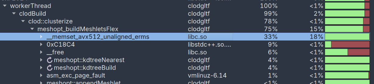
Rasterization:

Raytracing:

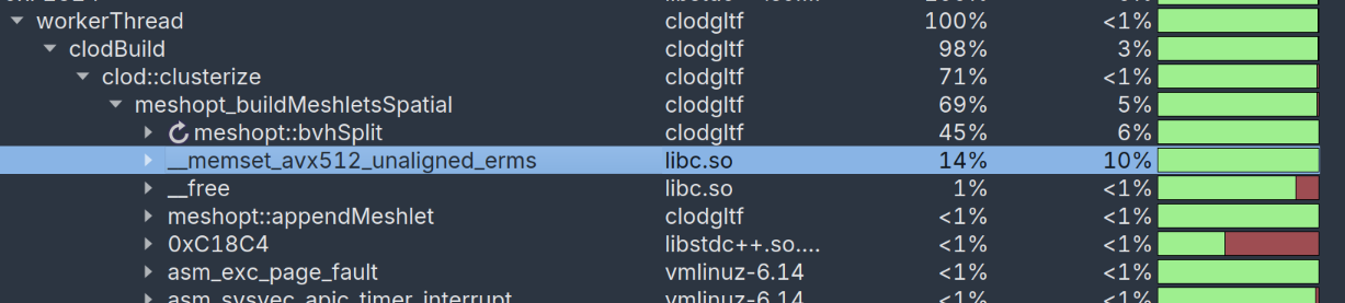
Hmm, that’s an awful lot of time to take for a memset! (we’ll come back to other issues here later)

What happens here is that both clusterizers use an array indexed by the vertex index to track whether a vertex is assigned to a current meshlet. This saves us the trouble of having to look through the 64-128 vertices when trying to see if adding a triangle to the meshlet would increase the vertex count. Unfortunately, this code:

memset(used, -1, vertex_count * sizeof(short));

… is only fast as long as the number of vertices is quite small - not so when we are repeatedly clusterizing subsets of a 30M triangle mesh! Curiously, a similar problem, but much less severe, existed in the simplifier too - as part of the work to make meshoptimizer friendlier towards clustered LOD use cases back in 2024, I’ve added a meshopt_SimplifySparse flag that assumes the input index buffer is a small subset of the mesh, and tries to avoid doing O(vertex_count) work at all costs… except that, too, had a small remaining issue, where it initialized a bit array for similar filtering:

memset(filter, 0, (vertex_count + 7) / 8);

Of course, 1 bit per vertex is much cheaper to fill than 16… but this still adds up when working with meshes approaching 100M triangles. Previously, the largest single mesh I’ve tested this code on was 6M triangles, 3M vertices - an order of magnitude smaller than individual meshes in this scene.

There are some ways to make this code more independent of the number of vertices - e.g. dynamically switch to a full hash map - but that carries extra costs and complexities, so for now let’s see what happens if we fix all of the issues by only initializing the array entries used by the index buffer when sparse access (index_count < vertex_count) is detected. Rerunning the code with these fixes⁵, we get 3m 31s for the raster version and 3m 57s for the raytrace version. Progress!

You will notice that the degree of the gains here does not align with the information the profiler is reporting. There are a few factors that contribute here, for example the profiler has significant overhead in this case which may skew the results; but more importantly, the time distribution the profiler is reporting is for all the work that happens across all threads, whereas the wall clock time for the entire processing depends on the slowest thread. Which brings us to…

Balancing threads

Instead of looking at the distribution of functions that take time, let’s instead focus on whether we are using threads well. When running the executable from the terminal, you can use /usr/bin/time -v to get the CPU% the command took; for us these are 1240-1260% depending on the mode we’re running at - in other words, we are using a little more than 12 threads’ worth of aggregate compute.

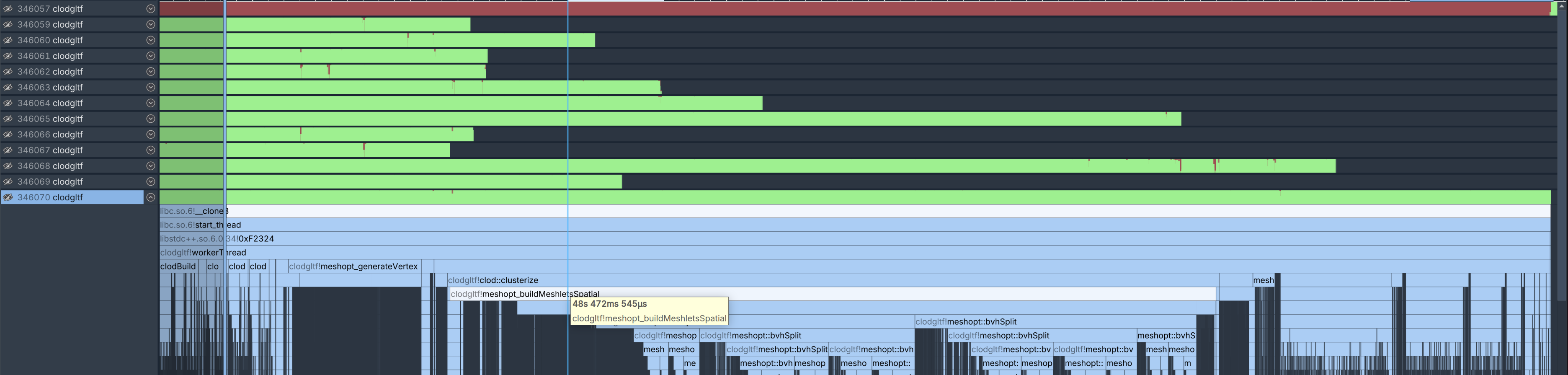
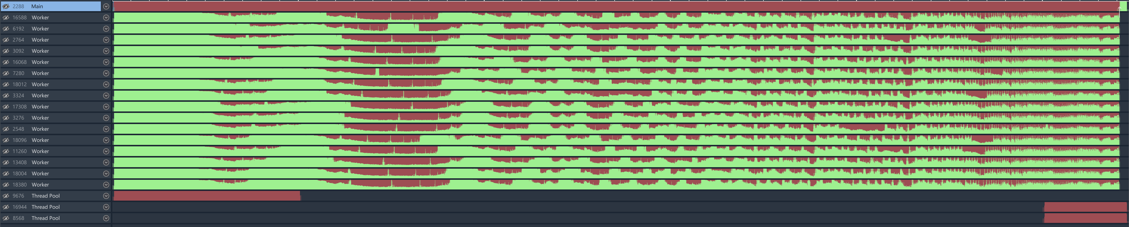
Let’s use Superluminal to look at the results more closely:

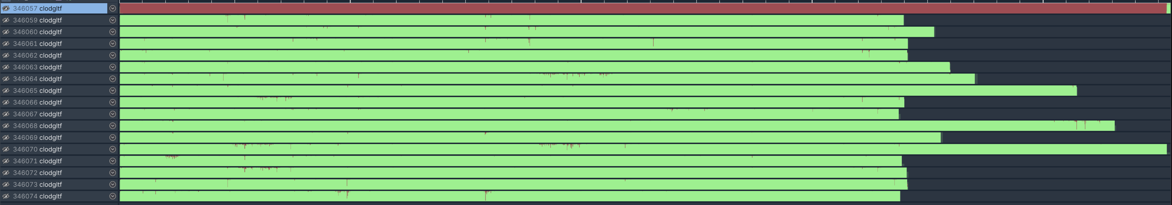
… ah yeah this is not great. If we look at the distribution for the number of triangles per mesh in this scene, we will see that there’s a significant imbalance: a few meshes are in the tens of millions of triangles, but most meshes don’t have as much. If we get unlucky, we may start processing large meshes much later into the process if they aren’t first in line to be queued for the thread pool; here we can see that in the “overhang”, there’s indeed a large mesh that takes ~48s to just build the clusters for the first DAG level. We need to be processing meshes like this first.

While fully general solutions to scheduling problems like this are very complicated and may or may not work well, fortunately we don’t need a general solution. The time it takes to process one mesh is a function of the number of triangles, so we can simply sort the meshes by triangle count in decreasing order. This ensures that we’ll process the most expensive meshes first.

This would also be a good time to mention the memory limits. Experimentally, we now know that it takes ~60 GB to process this scene on 16 threads - part of the reason why our processing is that much faster is that it takes less memory, allowing us to scale to more threads. However, what if the system we need to run on only has 40 GB RAM?⁶ Ideally, you’d use a limiter that only allows a certain fixed number of triangles to be processed “at once”; when running the next mesh, you could check if the total is at zero or under the limit, and wait until it goes below it to be safe. This can be implemented using a std::atomic (and yields/sleeps to avoid burning CPU power unnecessarily - although in this case it’s really a stopgap and we’d prefer to burn all the CPU power available to us thank you very much!), or a counting semaphore. Of course, for the purpose of this scene we’ll set the memory limit to be 60+ GB to make sure we don’t throttle the execution - 192 GB RAM is quite spacious after all.

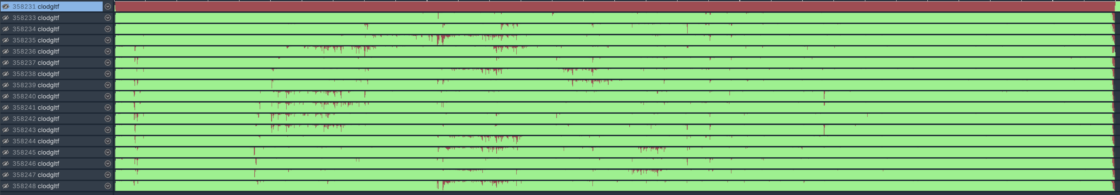
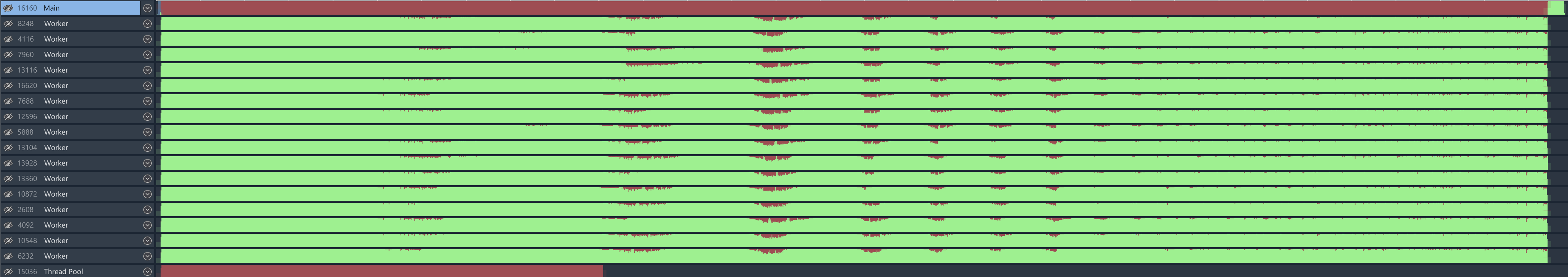
Anyhow, let’s sort the meshes and rerun the code. Here’s the new thread schedule:

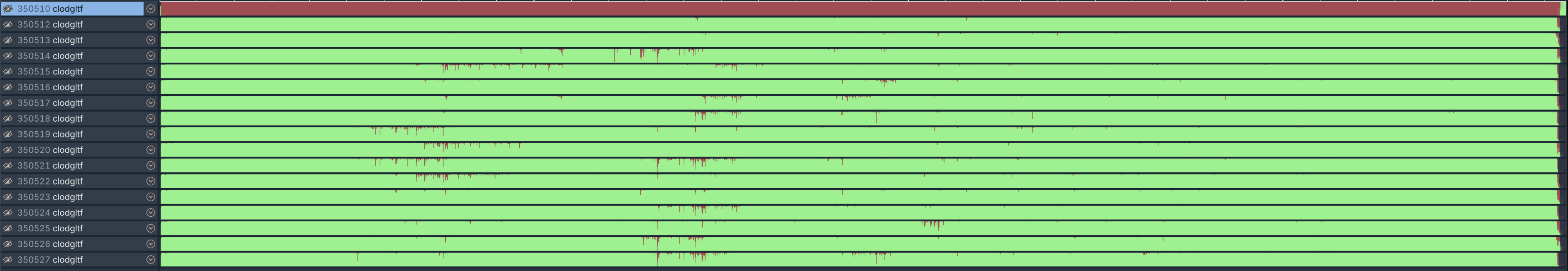
… sweet. While there are still a few little gaps here and there in the schedule, we now see the thread execution being perfectly balanced across 16 threads - /usr/bin/time reports 1574% CPU utilization. Front-loading large meshes means that smaller meshes can fill the gaps at the end fairly efficiently. Of course, if the input scene just has one or two meshes, our parallelism strategy will need to change - but for this scene, “external” parallelism where the axis is mesh count is the best as it allows us to share no data between different threads.

The execution time is now much better: 2m 56s for rasterization and 3m 07s for raytracing. Curiously, the peak memory consumption is actually a little lower (at ~45 GB for the raytracing version instead of ~54 GB before the sort). This is not very intuitive - normally you’d expect the peak memory consumption to be reached when each thread is processing the largest mesh which is what we’re doing here - but there’s probably some explanation that I’m missing right now; this will certainly depend on the particulars of the system allocator.

We’ve come quite a long way; ~3 minutes of processing time is quite a respectable number even though we’re not serializing the resulting data. That’s it then, see you next time!

Faster-er clusterization

… of course we’re not done. Coincidentally, right before NVIDIA had released the new asset files I’ve been working on performance improvements for both clusterizers. All of the results so far have been presented using meshoptimizer v0.25 (plus sparsity fixes), but actually we need to be testing on the latest master, which contains two important improvements to the clusterizer performance.

For the raster-optimized clusterizer, in some cases some internal tree searching functions would keep searching over the same data. I won’t go into too much detail as this post is getting long as it is, and it doesn’t affect these levels as acutely (saving ~3%); from now on, let’s focus on raytracing-optimized structures. Profiling the current code that takes ~3m 07s, we still see the new spatial clusterizer (meshopt_buildMeshletsSpatial) being responsible for two-thirds of the runtime. Fortunately, this is a case where we can point to a single function as the source of most of our problems:

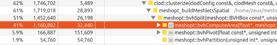
Conceptually, the core of the spatial clusterizer is quite close to a sweep BVH builder. For each level of the tree, we need to determine the best splitting plane; to do that, we need to analyze the cost of putting a splitting plane through the centroid of each triangle along each of the cardinal axes; that cost can be computed by accumulating the bounding boxes of the triangles six times - three axes times two directions, left and right; the resulting cost can be computed from the surface area of the resulting AABBs. While there’s much more to the algorithm itself, thankfully the complex external logic doesn’t contribute that much to the runtime.

void bvhComputeArea(float* areas, const BVHBox* boxes, const int* order, size_t count)
{
	BVHBox accuml = { {FLT_MAX, FLT_MAX, FLT_MAX}, {-FLT_MAX, -FLT_MAX, -FLT_MAX} };
	BVHBox accumr = accuml;

	for (size_t i = 0; i < count; ++i)
	{
		areas[i] = boxMerge(accuml, boxes[order[i]]);
		areas[i + count] = boxMerge(accumr, boxes[order[count - 1 - i]]);
	}
}

This case is a little curious because the performance characteristics of bvhComputeArea change at different levels of the processing, making analysis complicated. When clusterizing large meshes, initial calls to bvhSplit - which is a recursive function - end up processing the entire mesh with the locality of AABB traversal being Not Ideal. As such, we’d expect that function to be memory bound. When the recursive calls get all the way down to a few thousand triangles, the accesses become highly local because the “active” boxes readily fit into L2 and even L1.

The reason why this matters is that I initially thought I could improve this situation by reducing the amount of memory referenced by each box. However, this ended up not dramatically improving higher levels (presumably because the access locality was still poor) and regressing lower levels because storing AABBs in any other way than a few floats costs cycles to decode. After a few attempts to use different box representations, I gave up and tried a thing that should not have worked, which is to just convert the relevant code (boxMerge function used above) to SSE2. A box has two corners that can each be loaded into an SSE2 register; min/max accumulation can use dedicated MINPS/MAXPS instructions; and we can compute the box area by doing a moderate amount of shuffle crimes (in the absence of a dedicated DPPS instruction which requires SSE4.1). The same can then be done on NEON in case you are using ARM servers for content processing or for some strange reason running clustered raytracing acceleration code on a Mac.

The resulting SIMD code is quite straightforward and is only 20 lines of code per architecture. It’s not the world’s best SIMD code: we are only using 3 floats’ worth of computation even though the hardware could use much wider vectors, but unfortunately it’s difficult to rearrange the data to make the layout SIMD-optimal as the order of boxes has to change too frequently. Still, if we rerun the code, we go from 3m 07s to 2m 51s - ~9% speedup overall!⁷ This brings our raytracing-optimized code in line with rasterization-optimized, but we’re not quite done yet.

As mentioned, the earlier levels of the recursion are possibly hitting a memory subsystem limitation, as they end up bringing a lot of bounding boxes into the caches from all around the memory. It stands to reason that, if the bounding box order in memory - which matches the triangle order in the input index buffer - was more coherent, then we might see further speedup.

Indeed, what we can do is sort the triangles spatially, using a Morton order - conveniently, meshoptimizer provides a function that will do just that, meshopt_spatialSortTriangles. Calling this function has a cost - however, as long as the gains in clusterization time outweigh the extra effort to sort the triangles, this should still be a good idea. After trying this on that scene we get 2m 44s - ~5% further speedup for a single extra line. Nice!

Caching allocations

It’s time to tackle the final boss: all of the aforementioned functions need to allocate some memory for the processing. Given 16 threads that allocate sizeable chunks of memory, an ideal allocator would figure out how to keep some amount of memory in thread-local buffers to avoid allocations from one thread contending with allocations from another thread.

Unfortunately, expecting this may be overly optimistic, depending on the platform you’re running on. All of the experiments so far have been run on Linux (using the stock allocator without any extra configuration). And while in general we’re getting very reasonable performance with little contention, even on Linux there’s occasional “red” spots in the thread utilization chart, which indicates that the thread is busy waiting - and if we check, it’s indeed waiting on a different thread to service the allocation.

I’m a little hesitant to conclude specifics because under a heavy thread load, Superluminal offsets the timings enough that I worry about interference between the profiler and the results. However, we could instead switch to the platform where the stock allocator is not very high quality - Windows, and observe the bleak thread utilization picture:

What happens here is an unfortunate interaction between multi-threaded allocations and default large block policy. Large blocks bypass the heap and are allocated using VirtualAlloc; memory allocated this way is quite expensive to work with initially⁸, so repeat allocations/deallocations will cause performance problems. Because multiple threads contend over the same heap mutex, the resulting throughput is affected very significantly.

Fortunately, there’s a simple solution to this problem: just use a per-thread arena and route the allocations to it if they fit. meshoptimizer exposes an easy way to globally override the allocations, and guarantees that allocation/deallocation callbacks will be called in a stack-like manner. This makes it easy to implement a thread-local cache: pre-allocate a chunk of memory, say, 128 MB; allocate out of it using a bump allocator or fall back to malloc; deallocation can check if the pointer belongs to the thread-local arena and if it doesn’t, fall back to free.

Doing this on Linux provides modest further performance improvements; our code now runs in ~2m 35s - around 3.5x speedup from our initial baseline, and significantly better than ~30 minutes. On Windows, before this change, the code so far runs at 4m 20s - and with the thread cache we get 2m 38s, in line with our Linux version! And the utilization looks much better - note that we’re still using the global allocator for some STL code that’s part of the example (but can be replaced in the future), hence the imperfect utilization.

With some extra effort it’s possible to generalize the solution so that it’s easy to integrate on top of the default allocator; I’m planning to add this in a future meshoptimizer version, however since meshoptimizer will be 1.0 this year this will have to wait until the next version after that - in the meantime, the code is available under the MIT license.

Results

Are we done now? Well, more or less :) Most of the improvements, as well as a few improvements I didn’t think were of general enough interest to include, have been incorporated into the demo code that’s now distributed as a single-header “micro-library” via the meshoptimizer repository, clusterlod.h. The code is designed to be easy to modify and adapt, but also be easy to plug in as is.

Out of the aforementioned performance improvements, the call to meshopt_spatialSortTriangles can be made externally if necessary, and the thread cache work has not been submitted yet. It will likely be included into meshoptimizer after v1.0 is released later this year, as it’s generally useful for improving content pipeline performance, with or without clustered LOD.

And I thought this is more or less where things would end, but this example code has proven to be useful enough so that vk_lod_clusters, the sample that spawned all this work, integrates it as an option! You can select it by passing --nvclusterlod 0. The version that’s part of NVIDIA’s repository changes the example code to implement optional “internal” parallelism - being able to generate a cluster DAG from a single mesh using multiple threads. This is not something that is necessary for Zorah or other large scenes like this - as mentioned, “external” parallelism here provides a more natural and performant axis - but is crucial to be able to more quickly generate a DAG for a single large mesh.

Because of their work I can now show another screenshot of the same Zorah asset, but this time running inside the vk_lod_clusters sample using the data generated by meshoptimizer’s clusterlod.h, rendered with an approximately 2 GB geometry pool, in 26ms when using ray tracing and 16ms when using rasterization, on NVIDIA GeForce 3050. Not bad for a GPU that draws all its power from the motherboard without needing a separate power cable!

In vk_lod_clusters the processing is structured a little differently; as a result, it generates a slightly different amount of work compared to my simpler demo I’ve been using for profiling, and also includes data serialization, so it runs a little slower - ~3m 20s with all mentioned optimizations included. In that time it performs all the processing described above and generates the 62 GB cache file - including, hilariously, almost 10 seconds it takes Linux to fopen() this file for writing as it takes a while to discard the existing file contents from the file system cache, if present there! Since I’m also running my 7950X in eco mode, we’ll call it around 3 minutes, give or take.

There are still opportunities for improvement, however. Notably, to be able to stream and display a scene like this efficiently, you need a separate hierarchical acceleration structure that can quickly determine the set of clusters to render; vk_lod_clusters manages to do this using existing meshopt_ functions but that code is not part of clusterlod.h yet. Also the default cluster partitioning algorithm used in clusterlod.h to create groups of clusters is currently only willing to group clusters that are topologically adjacent (as in, they share vertices); this can sometimes result in DAGs that have too many roots, as the groups aren’t merged aggressively enough - and should be improved in the future as well (vk_lod_clusters falls back to a different meshopt_ partitioning algorithm if it detects this case).

But I’m happy to see a meaningful milestone for this code that started as a basic playground for clusterization algorithms.

Thanks to Christoph Kubisch for discussions, feedback and vk_lod_clusters integration, and to NVIDIA for sharing research, code and assets openly.